Back Arc Length and Metric Tensor To calculate the (squared) length of a vector, we take the dot product of the vector with it self:
∣ v ∣ 2 = v ⋅ v = ( v μ e μ ) ⋅ ( v ν e ν ) = v μ v ν ( e μ ⋅ e ν ) . \begin{align*} |\boldsymbol{v}|^2 &= \boldsymbol{v} \cdot \boldsymbol{v} \\ &= (v^{\mu} \boldsymbol{e_{\mu}}) \cdot (v^{\nu} \boldsymbol{e_{\nu}}) \\ &= v^{\mu} v^{\nu} (\boldsymbol{e_{\mu}} \cdot \boldsymbol{e_{\nu}}). \end{align*} ∣ v ∣ 2 = v ⋅ v = ( v μ e μ ) ⋅ ( v ν e ν ) = v μ v ν ( e μ ⋅ e ν ) . In 2D Cartesian coordinates, the dot products of basis vectors are as follows:
e x ⋅ e x = 1 , e x ⋅ e y = 0 , e y ⋅ e y = 1. \begin{align*} \boldsymbol{e_x} \cdot \boldsymbol{e_x} = 1, \\ \boldsymbol{e_x} \cdot \boldsymbol{e_y} = 0, \\ \boldsymbol{e_y} \cdot \boldsymbol{e_y} = 1. \end{align*} e x ⋅ e x = 1 , e x ⋅ e y = 0 , e y ⋅ e y = 1. The metric tensor g μ ν g_{\mu \nu} g μν
g μ ν = e μ ⋅ e ν . g_{\mu \nu} = \boldsymbol{e_{\mu}} \cdot \boldsymbol{e_{\nu}}. g μν = e μ ⋅ e ν . For the Cartesian coordinate system, the metric tensor is equal to the Kronecker delta:
g μ ν = δ μ ν = { 1 μ = ν , 0 μ ≠ ν , g_{\mu \nu} = \delta_{\mu \nu} = \begin{cases} 1 & \mu &= \nu, \\ 0 & \mu &\neq \nu, \end{cases} g μν = δ μν = { 1 0 μ μ = ν , = ν , Or represented as matrix for 2D Cartesian coordinate system:
g μ ν = [ 1 0 0 1 ] g_{\mu \nu} = \begin{bmatrix} 1 & 0 \\ 0 & 1 \end{bmatrix} g μν = [ 1 0 0 1 ] This means that the vectors are parallel to each other due to the missing off diagonal components.
The metric tensor has two covariant indices. Consider the coordinate transformation x μ → x ~ μ x^{\mu} \to \tilde{x}^{\mu} x μ → x ~ μ
e ~ μ = ∂ x ν ∂ x ~ μ e ν , \boldsymbol{\tilde{e}_{\mu}} = \frac{\partial x^{\nu}}{\partial \tilde{x}^{\mu}} \boldsymbol{e}_{\nu}, e ~ μ = ∂ x ~ μ ∂ x ν e ν , and the metric:
g ~ μ ν = e ~ μ ⋅ e ~ ν = ∂ x α ∂ x ~ μ e α ⋅ ∂ x β ∂ x ~ ν e β = ∂ x α ∂ x ~ μ ∂ x β ∂ x ~ ν e α ⋅ e β = ∂ x α ∂ x ~ μ ∂ x β ∂ x ~ ν g α β . \begin{align*} \tilde{g}_{\mu \nu} &= \boldsymbol{\tilde{e}_{\mu} \cdot \tilde{e}_{\nu}} \\ &= \frac{\partial x^{\alpha}}{\partial \tilde{x}^{\mu}} \boldsymbol{e}_{\alpha} \cdot \frac{\partial x^{\beta}}{\partial \tilde{x}^{\nu}} \boldsymbol{e}_{\beta} \\ &= \frac{\partial x^{\alpha}}{\partial \tilde{x}^{\mu}} \frac{\partial x^{\beta}}{\partial \tilde{x}^{\nu}} \boldsymbol{e}_{\alpha} \cdot \boldsymbol{e}_{\beta} \\ &= \frac{\partial x^{\alpha}}{\partial \tilde{x}^{\mu}} \frac{\partial x^{\beta}}{\partial \tilde{x}^{\nu}} g_{\alpha \beta}. \end{align*} g ~ μν = e ~ μ ⋅ e ~ ν = ∂ x ~ μ ∂ x α e α ⋅ ∂ x ~ ν ∂ x β e β = ∂ x ~ μ ∂ x α ∂ x ~ ν ∂ x β e α ⋅ e β = ∂ x ~ μ ∂ x α ∂ x ~ ν ∂ x β g α β . The metric tensor is also symmetric:
g μ ν = e μ ⋅ e ν = e ν ⋅ e μ = g ν μ . \begin{align*} g_{\mu \nu} &= \boldsymbol{e_{\mu}} \cdot \boldsymbol{e_{\nu}} \\ &= \boldsymbol{e_{\nu}} \cdot \boldsymbol{e_{\mu}} \\ &= g_{\nu \mu}. \end{align*} g μν = e μ ⋅ e ν = e ν ⋅ e μ = g νμ . Generally, if we want to compute the dot product of two vectors, we use the metric tensor:
v ⋅ w = ( v μ e μ ) ⋅ ( w ν e ν ) = v μ w ν ( e μ ⋅ e ν ) = v μ w ν g μ ν = ∣ v ∣ ∣ w ∣ cos θ , \begin{align*} \boldsymbol{v} \cdot \boldsymbol{w} &= (v^{\mu} \boldsymbol{e_{\mu}}) \cdot (w^{\nu} \boldsymbol{e_{\nu}}) \\ &= v^{\mu} w^{\nu} (\boldsymbol{e_{\mu}} \cdot \boldsymbol{e_{\nu}}) \\ &= v^{\mu} w^{\nu} g_{\mu \nu} = |\boldsymbol{v}| |\boldsymbol{w}| \cos \theta, \end{align*} v ⋅ w = ( v μ e μ ) ⋅ ( w ν e ν ) = v μ w ν ( e μ ⋅ e ν ) = v μ w ν g μν = ∣ v ∣∣ w ∣ cos θ , where θ \theta θ
The metric tensor is a function g : V × V → R g: V \times V \to \mathbb{R} g : V × V → R
g ( v , w ) = v μ w ν g μ ν . g(\boldsymbol{v}, \boldsymbol{w}) = v^{\mu} w^{\nu} g_{\mu \nu}. g ( v , w ) = v μ w ν g μν . We can scale the inputs of the metric tensor:
g ( a v , w ) = g ( v , a w ) = a g ( v , w ) , a ( v μ w ν g μ ν ) = ( a v μ ) w ν g μ ν = v μ ( a w ν ) g μ ν \begin{align*} g(a \boldsymbol{v}, \boldsymbol{w}) &= g(\boldsymbol{v}, a \boldsymbol{w}) = a g(\boldsymbol{v}, \boldsymbol{w}), \\ a (v^{\mu} w^{\nu} g_{\mu \nu}) &= (a v^{\mu}) w^{\nu} g_{\mu \nu} = v^{\mu} (a w^{\nu}) g_{\mu \nu} \end{align*} g ( a v , w ) a ( v μ w ν g μν ) = g ( v , a w ) = a g ( v , w ) , = ( a v μ ) w ν g μν = v μ ( a w ν ) g μν The inputs can also be added:
g ( v + u , w ) = g ( v , w ) + g ( u , w ) , ( v μ + u μ ) w ν g μ ν = v μ w ν g μ ν + u μ w ν g μ ν , g ( v , w + t ) = g ( v , w ) + g ( v , t ) , v μ ( w ν + t ν ) g μ ν = v μ w ν g μ ν + v μ t ν g μ ν , \begin{align*} g(\boldsymbol{v} + \boldsymbol{u}, \boldsymbol{w}) &= g(\boldsymbol{v}, \boldsymbol{w}) + g(\boldsymbol{u}, \boldsymbol{w}), \\ (v^{\mu} + u^{\mu}) w^{\nu} g_{\mu \nu} &= v^{\mu} w^{\nu} g_{\mu \nu} + u^{\mu} w^{\nu} g_{\mu \nu}, \\ g(\boldsymbol{v}, \boldsymbol{w} + \boldsymbol{t}) &= g(\boldsymbol{v}, \boldsymbol{w}) + g(\boldsymbol{v}, \boldsymbol{t}), \\ v^{\mu} (w^{\nu} + t^{\nu}) g_{\mu \nu} &= v^{\mu} w^{\nu} g_{\mu \nu} + v^{\mu} t^{\nu} g_{\mu \nu}, \end{align*} g ( v + u , w ) ( v μ + u μ ) w ν g μν g ( v , w + t ) v μ ( w ν + t ν ) g μν = g ( v , w ) + g ( u , w ) , = v μ w ν g μν + u μ w ν g μν , = g ( v , w ) + g ( v , t ) , = v μ w ν g μν + v μ t ν g μν , however:
g ( v + u , w + t ) ≠ g ( v , w ) + g ( u , t ) , g ( v + u , w + t ) = g ( v , w + t ) + g ( u , w + t ) = g ( v , w ) + g ( v , t ) + g ( u , w ) + g ( u , t ) . \begin{align*} g(\boldsymbol{v} + \boldsymbol{u}, \boldsymbol{w} + \boldsymbol{t}) &\neq g(\boldsymbol{v}, \boldsymbol{w}) + g(\boldsymbol{u}, \boldsymbol{t}), \\ g(\boldsymbol{v} + \boldsymbol{u}, \boldsymbol{w} + \boldsymbol{t}) &= g(\boldsymbol{v}, \boldsymbol{w} + \boldsymbol{t}) + g(\boldsymbol{u}, \boldsymbol{w} + \boldsymbol{t}) \\ &= g(\boldsymbol{v}, \boldsymbol{w}) + g(\boldsymbol{v}, \boldsymbol{t}) + g(\boldsymbol{u}, \boldsymbol{w}) + g(\boldsymbol{u}, \boldsymbol{t}). \end{align*} g ( v + u , w + t ) g ( v + u , w + t ) = g ( v , w ) + g ( u , t ) , = g ( v , w + t ) + g ( u , w + t ) = g ( v , w ) + g ( v , t ) + g ( u , w ) + g ( u , t ) . And this is the same definition as bilinear form:
B : V × V → R , a B ( v , w ) = B ( a v , w ) = B ( v , a w ) , B ( v + u , w ) = B ( v , w ) + B ( u , w ) , B ( v , w + t ) = B ( v , w ) + B ( v , t ) . \begin{gather*} \mathcal{B}: V \times V \to \mathbb{R}, \\ a\mathcal{B}(\boldsymbol{v}, \boldsymbol{w}) = \mathcal{B}(a\boldsymbol{v}, \boldsymbol{w}) = \mathcal{B}(\boldsymbol{v}, a\boldsymbol{w}), \\ \mathcal{B}(\boldsymbol{v} + \boldsymbol{u}, \boldsymbol{w}) = \mathcal{B}(\boldsymbol{v}, \boldsymbol{w}) + \mathcal{B}(\boldsymbol{u}, \boldsymbol{w}), \\ \mathcal{B}(\boldsymbol{v}, \boldsymbol{w} + \boldsymbol{t}) = \mathcal{B}(\boldsymbol{v}, \boldsymbol{w}) + \mathcal{B}(\boldsymbol{v}, \boldsymbol{t}). \end{gather*} B : V × V → R , a B ( v , w ) = B ( a v , w ) = B ( v , a w ) , B ( v + u , w ) = B ( v , w ) + B ( u , w ) , B ( v , w + t ) = B ( v , w ) + B ( v , t ) . The metric tensor is a bilinear form, but in addition it has two properties:
g ( v , w ) = g ( w , v ) , g ( v , v ) ≥ 0. \begin{align*} g(\boldsymbol{v}, \boldsymbol{w}) &= g(\boldsymbol{w}, \boldsymbol{v}), \tag{symmetricity} \\ g(\boldsymbol{v}, \boldsymbol{v}) &\geq 0. \tag{positive or zero length} \end{align*} g ( v , w ) g ( v , v ) = g ( w , v ) , ≥ 0. ( symmetricity ) ( positive or zero length ) A curve may be broken up into small pieces:
and if we sum over the lengths these small pieces, we get the arc length L L L
L ≈ ∑ i ∣ R ( λ + h ) − R ( λ ) ∣ L = lim h → 0 ∑ i ∣ R ( λ + h ) − R ( λ ) ∣ h h = ∫ ∣ d R d λ ∣ d λ , \begin{align*} L &\approx \sum_i |\boldsymbol{R}(\lambda + h) - \boldsymbol{R}(\lambda)| \\ L &= \lim_{h \to 0} \sum_i \frac{|\boldsymbol{R}(\lambda + h) - \boldsymbol{R}(\lambda)|}{h} h \\ &= \int \left|\frac{d\boldsymbol{R}}{d \lambda}\right| d\lambda, \end{align*} L L ≈ i ∑ ∣ R ( λ + h ) − R ( λ ) ∣ = h → 0 lim i ∑ h ∣ R ( λ + h ) − R ( λ ) ∣ h = ∫ d λ d R d λ , where d R d λ \frac{d\boldsymbol{R}}{d\lambda} d λ d R
∣ d R d λ ∣ 2 = d R d λ ⋅ d R d λ = ( ∂ R ∂ R μ d R μ d λ ) ⋅ ( ∂ R ∂ R ν d R ν d λ ) = d R μ d λ d R ν d λ ( ∂ R ∂ R μ ⋅ ∂ R ∂ R ν ) = d R μ d λ d R ν d λ ( e μ ⋅ e ν ) = d R μ d λ d R ν d λ g μ ν . \begin{align*} \left|\frac{d\boldsymbol{R}}{d \lambda}\right|^2 &= \frac{d \boldsymbol{R}}{d\lambda} \cdot \frac{d \boldsymbol{R}}{d\lambda} \\ &= \left(\frac{\partial \boldsymbol{R}}{\partial R^{\mu}} \frac{d R^{\mu}}{d \lambda}\right) \cdot \left(\frac{\partial \boldsymbol{R}}{\partial R^{\nu}} \frac{d R^{\nu}}{d \lambda}\right) \\ &= \frac{d R^{\mu}}{d \lambda} \frac{d R^{\nu}}{d \lambda} \left(\frac{\partial \boldsymbol{R}}{\partial R^{\mu}} \cdot \frac{\partial \boldsymbol{R}}{\partial R^{\nu}}\right) \\ &= \frac{d R^{\mu}}{d \lambda} \frac{d R^{\nu}}{d \lambda} \left(\boldsymbol{e_{\mu}} \cdot \boldsymbol{e_{\nu}}\right) \\ &= \frac{d R^{\mu}}{d \lambda} \frac{d R^{\nu}}{d \lambda} g_{\mu \nu}. \end{align*} d λ d R 2 = d λ d R ⋅ d λ d R = ( ∂ R μ ∂ R d λ d R μ ) ⋅ ( ∂ R ν ∂ R d λ d R ν ) = d λ d R μ d λ d R ν ( ∂ R μ ∂ R ⋅ ∂ R ν ∂ R ) = d λ d R μ d λ d R ν ( e μ ⋅ e ν ) = d λ d R μ d λ d R ν g μν . We would like to find a way to relate the vectors v \boldsymbol{v} v V V V V ∗ V^* V ∗ v \boldsymbol{v} v v ⋅ _ \boldsymbol{v} \cdot \_ v ⋅ _ _ \_ _ V ∗ V^* V ∗
v ⋅ _ : V → R , v ⋅ ( n a ) = n ( v ⋅ a ) , v ⋅ ( a + b ) = ( v ⋅ a ) + ( v ⋅ b ) , \begin{align*} \boldsymbol{v} \cdot \_: V \to \mathbb{R}, \\ \boldsymbol{v} \cdot (n\boldsymbol{a}) = n (\boldsymbol{v} \cdot \boldsymbol{a}), \\ \boldsymbol{v} \cdot (\boldsymbol{a} + \boldsymbol{b}) = (\boldsymbol{v} \cdot \boldsymbol{a}) + (\boldsymbol{v} \cdot \boldsymbol{b}), \end{align*} v ⋅ _ : V → R , v ⋅ ( n a ) = n ( v ⋅ a ) , v ⋅ ( a + b ) = ( v ⋅ a ) + ( v ⋅ b ) , and since it lives in the dual space V ∗ V^* V ∗
v ⋅ _ = v μ ϵ μ \boldsymbol{v} \cdot \_ = v_{\mu} \epsilon^{\mu} v ⋅ _ = v μ ϵ μ If we substitute w \boldsymbol{w} w v ⋅ _ \boldsymbol{v} \cdot \_ v ⋅ _
v ⋅ w = g ( v , w ) = g α β ϵ α ϵ β ( v γ e γ , w δ e δ ) = g α β ϵ α ( v γ e γ ) ϵ β ( w δ e δ ) = g α β v γ w δ ϵ α ( e γ ) ϵ β ( e δ ) = g α β v γ w δ δ γ α δ δ β = g α β v α w β \begin{align*} \boldsymbol{v} \cdot \boldsymbol{w} &= g(\boldsymbol{v}, \boldsymbol{w}) \\ &= g_{\alpha \beta} \epsilon^{\alpha} \epsilon^{\beta} (v^{\gamma} \boldsymbol{e_{\gamma}}, w^{\delta} \boldsymbol{e_{\delta}}) \\ &= g_{\alpha \beta} \epsilon^{\alpha} (v^{\gamma} \boldsymbol{e_{\gamma}}) \epsilon^{\beta} (w^{\delta} \boldsymbol{e_{\delta}}) \\ &= g_{\alpha \beta} v^{\gamma} w^{\delta} \epsilon^{\alpha} (\boldsymbol{e_{\gamma}}) \epsilon^{\beta} (\boldsymbol{e_{\delta}}) \\ &= g_{\alpha \beta} v^{\gamma} w^{\delta} \delta^{\alpha}_{\gamma} \delta^{\beta}_{\delta} \\ &= g_{\alpha \beta} v^{\alpha} w^{\beta} \end{align*} v ⋅ w = g ( v , w ) = g α β ϵ α ϵ β ( v γ e γ , w δ e δ ) = g α β ϵ α ( v γ e γ ) ϵ β ( w δ e δ ) = g α β v γ w δ ϵ α ( e γ ) ϵ β ( e δ ) = g α β v γ w δ δ γ α δ δ β = g α β v α w β we arrive at the formula for dot product. If we instead not substitute anything and consider just v ⋅ _ \boldsymbol{v} \cdot \_ v ⋅ _
v ⋅ _ = g ( v , _ ) = g α β ϵ α ϵ β ( v γ e γ ) = g α β v γ ϵ α ϵ β ( e γ ) = g α β v γ ϵ α δ γ β = g α β v β ϵ α . \begin{align*} \boldsymbol{v} \cdot \_ &= g(\boldsymbol{v}, \_) \\ &= g_{\alpha \beta} \epsilon^{\alpha} \epsilon^{\beta} (v^{\gamma} \boldsymbol{e_{\gamma}}) \\ &= g_{\alpha \beta} v^{\gamma} \epsilon^{\alpha} \epsilon^{\beta} (\boldsymbol{e_{\gamma}}) \\ &= g_{\alpha \beta} v^{\gamma} \epsilon^{\alpha} \delta^{\beta}_{\gamma} \\ &= g_{\alpha \beta} v^{\beta} \epsilon^{\alpha}. \end{align*} v ⋅ _ = g ( v , _ ) = g α β ϵ α ϵ β ( v γ e γ ) = g α β v γ ϵ α ϵ β ( e γ ) = g α β v γ ϵ α δ γ β = g α β v β ϵ α . This is the component decomposition of v ⋅ _ \boldsymbol{v} \cdot \_ v ⋅ _ g α β v β g_{\alpha \beta} v^{\beta} g α β v β v α v_{\alpha} v α
v α = g α β v β , v ⋅ _ = v α ϵ α = g α β v β ϵ α . \begin{align*} v_{\alpha} &= g_{\alpha \beta} v^{\beta}, \\ \boldsymbol{v} \cdot \_ &= v_{\alpha} \epsilon^{\alpha} = g_{\alpha \beta} v^{\beta} \epsilon^{\alpha}. \end{align*} v α v ⋅ _ = g α β v β , = v α ϵ α = g α β v β ϵ α . Generally v μ ≠ v μ v_{\mu} \neq v^{\mu} v μ = v μ
We can lower an index. Now we need to figure out how to raise an index. For this, we will use the inverse metric g μ ν g^{\mu \nu} g μν
g α β g β γ = δ γ α . g^{\alpha \beta} g_{\beta \gamma} = \delta^{\alpha}_{\gamma}. g α β g β γ = δ γ α . The equation for covector components v α = g α β v β v_{\alpha} = g_{\alpha \beta} v^{\beta} v α = g α β v β g γ α g^{\gamma \alpha} g γ α
g γ α v α = g γ α g α β v β = δ β γ v β = v γ . \begin{align*} g^{\gamma \alpha} v_{\alpha} &= g^{\gamma \alpha} g_{\alpha \beta} v^{\beta} \\ &= \delta^{\gamma}_{\beta} v^{\beta} \\ &= v^{\gamma}. \end{align*} g γ α v α = g γ α g α β v β = δ β γ v β = v γ . So to summarize:
v μ = g μ ν v ν , v μ = g μ ν v ν . \begin{align*} v_{\mu} &= g_{\mu \nu} v^{\nu}, \\ v^{\mu} &= g^{\mu \nu} v_{\nu}. \end{align*} v μ v μ = g μν v ν , = g μν v ν . Consider a point parametrized by the distance from the origin r r r θ \theta θ
From the diagram we can see:
x = r cos θ , y = r sin θ . \begin{align*} x &= r \cos \theta, \\ y &= r \sin \theta. \end{align*} x y = r cos θ , = r sin θ . The partial derivatives are:
∂ x ∂ r = cos θ , ∂ x ∂ θ = − r sin θ , ∂ y ∂ r = sin θ , ∂ y ∂ θ = r cos θ . \begin{align*} \frac{\partial x}{\partial r} &= \cos \theta, & \frac{\partial x}{\partial \theta} &= -r \sin \theta, \\ \frac{\partial y}{\partial r} &= \sin \theta, & \frac{\partial y}{\partial \theta} &= r \cos \theta. \end{align*} ∂ r ∂ x ∂ r ∂ y = cos θ , = sin θ , ∂ θ ∂ x ∂ θ ∂ y = − r sin θ , = r cos θ . The metric tensor in 2D Cartesian coordinates is the Kronecker delta δ μ ν \delta_{\mu \nu} δ μν g ~ μ ν \tilde{g}_{\mu \nu} g ~ μν
g ~ μ ν = ∂ x α ∂ x μ ∂ x β ∂ x ν g α β = ∂ x α ∂ x μ ∂ x β ∂ x ν δ α β = ∑ α ∂ x α ∂ x μ ∂ x α ∂ x ν . \begin{align*} \tilde{g}_{\mu \nu} &= \frac{\partial x^{\alpha}}{\partial x^{\mu}} \frac{\partial x^{\beta}}{\partial x^{\nu}} g_{\alpha \beta} \\ &= \frac{\partial x^{\alpha}}{\partial x^{\mu}} \frac{\partial x^{\beta}}{\partial x^{\nu}} \delta_{\alpha \beta} \\ &= \sum_{\alpha} \frac{\partial x^{\alpha}}{\partial x^{\mu}} \frac{\partial x^{\alpha}}{\partial x^{\nu}}. \end{align*} g ~ μν = ∂ x μ ∂ x α ∂ x ν ∂ x β g α β = ∂ x μ ∂ x α ∂ x ν ∂ x β δ α β = α ∑ ∂ x μ ∂ x α ∂ x ν ∂ x α . The components of the polar metric tensor are equal to:
g ~ r r = ∑ α ∂ x α ∂ r ∂ x α ∂ r = cos 2 θ + sin 2 θ = 1 , g ~ r θ = g ~ θ r = ∑ α ∂ x α ∂ r ∂ x α ∂ θ = − r cos θ sin θ + r sin θ cos θ = 0 , g ~ θ θ = ∑ α ∂ x α ∂ θ ∂ x α ∂ θ = ( − r sin θ ) 2 + ( r cos θ ) 2 = r 2 sin 2 θ + r 2 cos 2 θ = r 2 , \begin{align*} \tilde{g}_{rr} &= \sum_{\alpha} \frac{\partial x^{\alpha}}{\partial r} \frac{\partial x^{\alpha}}{\partial r} \\ &= \cos^2 \theta + \sin^2 \theta \\ &= 1, \\ \tilde{g}_{r \theta} = \tilde{g}_{\theta r} &= \sum_{\alpha} \frac{\partial x^{\alpha}}{\partial r} \frac{\partial x^{\alpha}}{\partial \theta} \\ &= -r \cos \theta \sin \theta + r \sin \theta \cos \theta \\ &= 0, \\ \tilde{g}_{\theta \theta} &= \sum_{\alpha} \frac{\partial x^{\alpha}}{\partial \theta} \frac{\partial x^{\alpha}}{\partial \theta} \\ &= (-r \sin \theta)^2 + (r \cos \theta)^2 \\ &= r^2 \sin^2 \theta + r^2 \cos^2 \theta \\ &= r^2, \end{align*} g ~ rr g ~ r θ = g ~ θ r g ~ θθ = α ∑ ∂ r ∂ x α ∂ r ∂ x α = cos 2 θ + sin 2 θ = 1 , = α ∑ ∂ r ∂ x α ∂ θ ∂ x α = − r cos θ sin θ + r sin θ cos θ = 0 , = α ∑ ∂ θ ∂ x α ∂ θ ∂ x α = ( − r sin θ ) 2 + ( r cos θ ) 2 = r 2 sin 2 θ + r 2 cos 2 θ = r 2 , or in matrix notation:
g ~ μ ν = [ 1 0 0 r 2 ] . \tilde{g}_{\mu \nu} = \begin{bmatrix} 1 & 0 \\ 0 & r^2 \end{bmatrix}. g ~ μν = [ 1 0 0 r 2 ] . Consider the spherical coordinates where the coordinates are: r r r θ \theta θ ϕ \phi ϕ
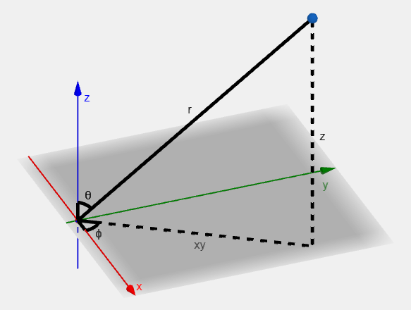
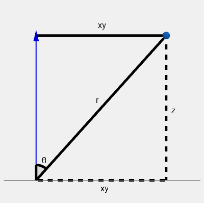
We can start by solving for the cartesian coordinate z z z x y xy x y x - y x\textrm{-}y x - y
z = r cos θ , x y = r sin θ . \begin{align*} z &= r \cos \theta, \\ xy &= r \sin \theta. \end{align*} z x y = r cos θ , = r sin θ . And now we can solve fot the Cartesian coordinates x x x y y y
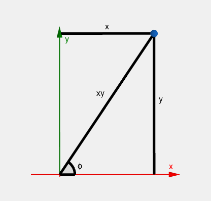
x = x y cos ϕ = r cos ϕ sin θ , y = x y sin ϕ = r sin ϕ sin θ . \begin{align*} x &= xy \cos \phi = r \cos \phi \sin \theta, \\ y &= xy \sin \phi = r \sin \phi \sin \theta. \\ \end{align*} x y = x y cos ϕ = r cos ϕ sin θ , = x y sin ϕ = r sin ϕ sin θ . Putting it all together, the Cartesian coordinates with the cartesian metric tensor g μ ν g_{\mu \nu} g μν
x = r sin θ cos ϕ , y = r sin θ sin ϕ , z = r cos θ , g μ ν = δ μ ν = [ 1 0 0 0 1 0 0 0 1 ] . \begin{align*} x &= r \sin \theta \cos \phi, \\ y &= r \sin \theta \sin \phi, \\ z &= r \cos \theta, \\ g_{\mu \nu} &= \delta_{\mu \nu} = \begin{bmatrix} 1 & 0 & 0 \\ 0 & 1 & 0 \\ 0 & 0 & 1 \end{bmatrix}. \end{align*} x y z g μν = r sin θ cos ϕ , = r sin θ sin ϕ , = r cos θ , = δ μν = 1 0 0 0 1 0 0 0 1 . The metric tensor g ~ μ ν \tilde{g}_{\mu \nu} g ~ μν
g ~ μ ν = ∂ x α ∂ x ~ μ ∂ x β ∂ x ~ ν g α β = ∂ x α ∂ x ~ μ ∂ x β ∂ x ~ ν δ α β = ∑ α ∂ x α ∂ x ~ μ ∂ x α ∂ x ~ ν . \begin{align*} \tilde{g}_{\mu \nu} &= \frac{\partial x^{\alpha}}{\partial \tilde{x}^{\mu}} \frac{\partial x^{\beta}}{\partial \tilde{x}^{\nu}} g_{\alpha \beta} \\ &= \frac{\partial x^{\alpha}}{\partial \tilde{x}^{\mu}} \frac{\partial x^{\beta}}{\partial \tilde{x}^{\nu}} \delta_{\alpha \beta} \\ &= \sum_{\alpha} \frac{\partial x^{\alpha}}{\partial \tilde{x}^{\mu}} \frac{\partial x^{\alpha}}{\partial \tilde{x}^{\nu}}. \end{align*} g ~ μν = ∂ x ~ μ ∂ x α ∂ x ~ ν ∂ x β g α β = ∂ x ~ μ ∂ x α ∂ x ~ ν ∂ x β δ α β = α ∑ ∂ x ~ μ ∂ x α ∂ x ~ ν ∂ x α . The partial derivatives in the transformation are equal to:
∂ x ∂ r = sin θ cos ϕ , ∂ x ∂ θ = r cos θ cos ϕ , ∂ x ∂ ϕ = − r sin θ sin ϕ , ∂ y ∂ r = sin θ sin ϕ , ∂ y ∂ θ = r cos θ sin ϕ , ∂ y ∂ ϕ = r sin θ cos ϕ , ∂ z ∂ r = cos θ , ∂ z ∂ θ = − r sin θ , ∂ z ∂ ϕ = 0. \begin{align*} \frac{\partial x}{\partial r} &= \sin \theta \cos \phi, & \frac{\partial x}{\partial \theta} &= r \cos \theta \cos \phi, & \frac{\partial x}{\partial \phi} &= -r \sin \theta \sin \phi, \\ \frac{\partial y}{\partial r} &= \sin \theta \sin \phi, & \frac{\partial y}{\partial \theta} &= r \cos \theta \sin \phi, & \frac{\partial y}{\partial \phi} &= r \sin \theta \cos \phi, \\ \frac{\partial z}{\partial r} &= \cos \theta, & \frac{\partial z}{\partial \theta} &= -r \sin \theta, & \frac{\partial z}{\partial \phi} &= 0. \end{align*} ∂ r ∂ x ∂ r ∂ y ∂ r ∂ z = sin θ cos ϕ , = sin θ sin ϕ , = cos θ , ∂ θ ∂ x ∂ θ ∂ y ∂ θ ∂ z = r cos θ cos ϕ , = r cos θ sin ϕ , = − r sin θ , ∂ ϕ ∂ x ∂ ϕ ∂ y ∂ ϕ ∂ z = − r sin θ sin ϕ , = r sin θ cos ϕ , = 0. Transforming the metric tensor components:
g ~ r r = ∑ α ∂ x α ∂ r ∂ x α ∂ r = ( sin θ cos ϕ ) 2 + ( sin θ sin ϕ ) 2 + ( cos θ ) 2 = sin 2 θ cos 2 ϕ + sin 2 θ sin 2 ϕ + cos 2 θ = sin 2 θ + cos 2 θ = 1 , g ~ r θ = g ~ θ r = ∑ α ∂ x α ∂ r ∂ x α ∂ θ = sin θ cos ϕ r cos θ cos ϕ + sin θ sin ϕ r cos θ sin ϕ − cos θ r sin θ = r sin θ cos θ ( cos 2 ϕ + sin 2 ϕ ) − r sin θ cos θ = r sin θ cos θ − r sin θ cos θ = 0 , g ~ r ϕ = g ~ ϕ r = ∑ α ∂ x α ∂ r ∂ x α ∂ ϕ = − sin θ cos ϕ r sin θ sin ϕ + sin θ sin ϕ r sin θ cos ϕ + cos θ 0 = − sin θ cos ϕ r sin θ sin ϕ + sin θ sin ϕ r sin θ cos ϕ + cos θ 0 = 0 , g ~ θ θ = ∑ α ∂ x α ∂ θ ∂ x α ∂ θ = ( r cos θ cos ϕ ) 2 + ( r cos θ sin ϕ ) 2 + ( − r sin θ ) 2 = r 2 cos 2 θ cos 2 ϕ + r 2 cos 2 θ sin 2 ϕ + r 2 sin 2 θ = r 2 cos 2 θ ( cos 2 ϕ + sin 2 ϕ ) + r 2 sin 2 θ = r 2 cos 2 θ + r 2 sin 2 θ = r 2 g ~ θ ϕ = g ~ ϕ θ = ∑ α ∂ x α ∂ θ ∂ x α ∂ ϕ = − r cos θ cos ϕ r sin θ sin ϕ + r cos θ sin ϕ r sin θ cos ϕ − r sin θ 0 = 0 , g ~ ϕ ϕ = ∑ α ∂ x α ∂ ϕ ∂ x α ∂ ϕ = ( − r sin θ sin ϕ ) 2 + ( r sin θ cos ϕ ) 2 + 0 2 = r 2 sin 2 θ sin 2 ϕ + r 2 sin 2 θ cos 2 ϕ = r 2 sin 2 θ ( sin 2 ϕ + cos 2 ϕ ) = r 2 sin 2 θ , \begin{align*} \tilde{g}_{r r} &= \sum_{\alpha} \frac{\partial x^{\alpha}}{\partial r} \frac{\partial x^{\alpha}}{\partial r} \\ &= (\sin \theta \cos \phi)^2 + (\sin \theta \sin \phi)^2 + (\cos \theta)^2 \\ &= \sin^2 \theta \cos^2 \phi + \sin^2 \theta \sin^2 \phi + \cos^2 \theta \\ &= \sin^2 \theta + \cos^2 \theta \\ &= 1, \\ \tilde{g}_{r \theta} = \tilde{g}_{\theta r} &= \sum_{\alpha} \frac{\partial x^{\alpha}}{\partial r} \frac{\partial x^{\alpha}}{\partial \theta} \\ &= \sin \theta \cos \phi\ r \cos \theta \cos \phi + \sin \theta \sin \phi\ r \cos \theta \sin \phi - \cos \theta\ r \sin \theta \\ &= r \sin \theta \cos \theta (\cos^2 \phi + \sin^2 \phi) - r \sin \theta \cos \theta \\ &= r \sin \theta \cos \theta - r \sin \theta \cos \theta \\ &= 0, \\ \tilde{g}_{r \phi} = \tilde{g}_{\phi r} &= \sum_{\alpha} \frac{\partial x^{\alpha}}{\partial r} \frac{\partial x^{\alpha}}{\partial \phi} \\ &= -\sin \theta \cos \phi\ r \sin \theta \sin \phi + \sin \theta \sin \phi\ r \sin \theta \cos \phi + \cos \theta\ 0 \\ &= -\sin \theta \cos \phi\ r \sin \theta \sin \phi + \sin \theta \sin \phi\ r \sin \theta \cos \phi + \cos \theta\ 0 \\ &= 0, \\ \tilde{g}_{\theta \theta} &= \sum_{\alpha} \frac{\partial x^{\alpha}}{\partial \theta} \frac{\partial x^{\alpha}}{\partial \theta} \\ &= (r \cos \theta \cos \phi)^2 + (r \cos \theta \sin \phi)^2 + (- r \sin \theta)^2 \\ &= r^2 \cos^2 \theta \cos^2 \phi + r^2 \cos^2 \theta \sin^2 \phi + r^2 \sin^2 \theta \\ &= r^2 \cos^2 \theta (\cos^2 \phi + \sin^2 \phi) + r^2 \sin^2 \theta \\ &= r^2 \cos^2 \theta + r^2 \sin^2 \theta \\ &= r^2 \\ \tilde{g}_{\theta \phi} = \tilde{g}_{\phi \theta} &= \sum_{\alpha} \frac{\partial x^{\alpha}}{\partial \theta} \frac{\partial x^{\alpha}}{\partial \phi} \\ &= -r \cos \theta \cos \phi\ r \sin \theta \sin \phi + r \cos \theta \sin \phi\ r \sin \theta \cos \phi - r \sin \theta\ 0 \\ &= 0, \\ \tilde{g}_{\phi \phi} &= \sum_{\alpha} \frac{\partial x^{\alpha}}{\partial \phi} \frac{\partial x^{\alpha}}{\partial \phi} \\ &= (- r \sin \theta \sin \phi)^2 + (r \sin \theta \cos \phi)^2 + 0^2 \\ &= r^2 \sin^2 \theta \sin^2 \phi + r^2 \sin^2 \theta \cos^2 \phi \\ &= r^2 \sin^2 \theta (\sin^2 \phi + \cos^2 \phi) \\ &= r^2 \sin^2 \theta, \end{align*} g ~ rr g ~ r θ = g ~ θ r g ~ r ϕ = g ~ ϕ r g ~ θθ g ~ θϕ = g ~ ϕθ g ~ ϕϕ = α ∑ ∂ r ∂ x α ∂ r ∂ x α = ( sin θ cos ϕ ) 2 + ( sin θ sin ϕ ) 2 + ( cos θ ) 2 = sin 2 θ cos 2 ϕ + sin 2 θ sin 2 ϕ + cos 2 θ = sin 2 θ + cos 2 θ = 1 , = α ∑ ∂ r ∂ x α ∂ θ ∂ x α = sin θ cos ϕ r cos θ cos ϕ + sin θ sin ϕ r cos θ sin ϕ − cos θ r sin θ = r sin θ cos θ ( cos 2 ϕ + sin 2 ϕ ) − r sin θ cos θ = r sin θ cos θ − r sin θ cos θ = 0 , = α ∑ ∂ r ∂ x α ∂ ϕ ∂ x α = − sin θ cos ϕ r sin θ sin ϕ + sin θ sin ϕ r sin θ cos ϕ + cos θ 0 = − sin θ cos ϕ r sin θ sin ϕ + sin θ sin ϕ r sin θ cos ϕ + cos θ 0 = 0 , = α ∑ ∂ θ ∂ x α ∂ θ ∂ x α = ( r cos θ cos ϕ ) 2 + ( r cos θ sin ϕ ) 2 + ( − r sin θ ) 2 = r 2 cos 2 θ cos 2 ϕ + r 2 cos 2 θ sin 2 ϕ + r 2 sin 2 θ = r 2 cos 2 θ ( cos 2 ϕ + sin 2 ϕ ) + r 2 sin 2 θ = r 2 cos 2 θ + r 2 sin 2 θ = r 2 = α ∑ ∂ θ ∂ x α ∂ ϕ ∂ x α = − r cos θ cos ϕ r sin θ sin ϕ + r cos θ sin ϕ r sin θ cos ϕ − r sin θ 0 = 0 , = α ∑ ∂ ϕ ∂ x α ∂ ϕ ∂ x α = ( − r sin θ sin ϕ ) 2 + ( r sin θ cos ϕ ) 2 + 0 2 = r 2 sin 2 θ sin 2 ϕ + r 2 sin 2 θ cos 2 ϕ = r 2 sin 2 θ ( sin 2 ϕ + cos 2 ϕ ) = r 2 sin 2 θ , or in matrix notation:
g ~ μ ν = [ 1 0 0 0 r 2 0 0 0 r 2 sin 2 θ ] . \tilde{g}_{\mu \nu} = \begin{bmatrix} 1 & 0 & 0 \\ 0 & r^2 & 0 \\ 0 & 0 & r^2 \sin^2 \theta \\ \end{bmatrix}. g ~ μν = 1 0 0 0 r 2 0 0 0 r 2 sin 2 θ . In this section, I will refer to the spherical metric tensor as g μ ν g_{\mu \nu} g μν
g μ ν = [ 1 0 0 0 r 2 0 0 0 r 2 sin 2 θ ] . g_{\mu \nu} = \begin{bmatrix} 1 & 0 & 0 \\ 0 & r^2 & 0 \\ 0 & 0 & r^2 \sin^2 \theta \\ \end{bmatrix}. g μν = 1 0 0 0 r 2 0 0 0 r 2 sin 2 θ . By keeping r r r
To represent coordinates, we choose a 2D θ - ϕ \theta\textrm{-}\phi θ - ϕ θ \theta θ ϕ \phi ϕ
where 0 ≤ θ ≤ π 0 \leq \theta \leq \pi 0 ≤ θ ≤ π 0 ≤ ϕ ≤ 2 π 0 \leq \phi \leq 2\pi 0 ≤ ϕ ≤ 2 π
Consider a curve parametrized in the ϕ - θ \phi\textrm{-}\theta ϕ - θ
θ ( λ ) = λ , ϕ ( λ ) = λ , 0 ≤ λ ≤ π . \begin{align*} \theta(\lambda) &= \lambda, \\ \phi(\lambda) &= \lambda, \\ 0 \leq \lambda &\leq \pi. \end{align*} θ ( λ ) ϕ ( λ ) 0 ≤ λ = λ , = λ , ≤ π . Rendering, on our plane, the curve looks like this:
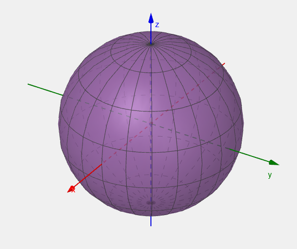
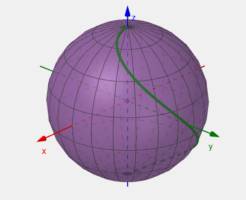
However, on the sphere, the curve looks like this:
We could naively calculate the length of the curve from the plane using Pythagorean theorem:
s = ϕ 2 + θ 2 = π 2 + π 2 = π 2 . s = \sqrt{\phi^2 + \theta^2} = \sqrt{\pi^2 + \pi^2} = \pi \sqrt{2}. s = ϕ 2 + θ 2 = π 2 + π 2 = π 2 . However, we always have to use the metric tensor:
s = ∫ 0 π ∣ d R d λ ∣ d λ = ∫ 0 π g μ ν d R μ d λ d R ν d λ d λ = ∫ 0 π g μ μ ( d R μ d λ ) 2 d λ = ∫ 0 π ( d r d λ ) 2 + r 2 ( d θ d λ ) 2 + r 2 sin 2 θ ( d ϕ d λ ) 2 d λ = ∫ 0 π r 2 + r 2 sin 2 θ d λ = r 2 ∫ 0 π 1 + sin 2 λ d λ ≈ 3.8202 r 2 ≠ π 2 . \begin{align*} s &= \int_0^{\pi} \left|\frac{d \boldsymbol{R}}{d \lambda}\right| d\lambda \\ &= \int_0^{\pi} \sqrt{g_{\mu \nu} \frac{d R^{\mu}}{d \lambda} \frac{d R^{\nu}}{d \lambda}} d\lambda \\ &= \int_0^{\pi} \sqrt{g_{\mu \mu} \left(\frac{d R^{\mu}}{d \lambda}\right)^2} d\lambda \\ &= \int_0^{\pi} \sqrt{\left(\frac{d r}{d \lambda}\right)^2 + r^2 \left(\frac{d \theta}{d \lambda}\right)^2 + r^2 \sin^2 \theta \left(\frac{d \phi}{d \lambda}\right)^2} d\lambda \\ &= \int_0^{\pi} \sqrt{r^2 + r^2 \sin^2 \theta} d\lambda \\ &= r^2 \int_0^{\pi} \sqrt{1 + \sin^2 \lambda}\ d\lambda \\ &\approx 3.8202 r^2 \neq \pi \sqrt{2}. \end{align*} s = ∫ 0 π d λ d R d λ = ∫ 0 π g μν d λ d R μ d λ d R ν d λ = ∫ 0 π g μμ ( d λ d R μ ) 2 d λ = ∫ 0 π ( d λ d r ) 2 + r 2 ( d λ d θ ) 2 + r 2 sin 2 θ ( d λ d ϕ ) 2 d λ = ∫ 0 π r 2 + r 2 sin 2 θ d λ = r 2 ∫ 0 π 1 + sin 2 λ d λ ≈ 3.8202 r 2 = π 2 . This is the extrinsic metric tensor - to work with 2D surface, we need three dimensions. To calculate curve lengths on the surface as if we are living on it (similar to Earth), we need to define an intrinsic metric tensor g ˉ μ ν \bar{g}_{\mu \nu} g ˉ μν
To start, consider again a vector R \boldsymbol{R} R
d R d λ = d R μ d λ ∂ R ∂ R μ = d R μ d λ e ˉ μ , \frac{d \boldsymbol{R}}{d\lambda} = \frac{d R^{\mu}}{d \lambda} \frac{\partial \boldsymbol{R}}{\partial R^{\mu}} = \frac{d R^{\mu}}{d \lambda} \boldsymbol{\bar{e}_{\mu}}, d λ d R = d λ d R μ ∂ R μ ∂ R = d λ d R μ e ˉ μ , where e ˉ μ \boldsymbol{\bar{e}_{\mu}} e ˉ μ e ˉ θ \boldsymbol{\bar{e}_{\theta}} e ˉ θ e ˉ ϕ \boldsymbol{\bar{e}_{\phi}} e ˉ ϕ R \boldsymbol{R} R
d d λ = d x ˉ μ d λ ∂ ∂ x ˉ μ = d x ˉ μ d λ e ˉ μ , \frac{d}{d\lambda} = \frac{d \bar{x}^{\mu}}{d \lambda} \frac{\partial}{\partial \bar{x}^{\mu}} = \frac{d \bar{x}^{\mu}}{d \lambda} \boldsymbol{\bar{e}_{\mu}}, d λ d = d λ d x ˉ μ ∂ x ˉ μ ∂ = d λ d x ˉ μ e ˉ μ , The squared length of the tangent vector is given by:
∣ d d λ ∣ 2 = ( d x ˉ μ d λ e ˉ μ ) ⋅ ( d x ˉ ν d λ e ˉ ν ) = d x ˉ μ d λ d x ˉ ν d λ g ˉ μ ν . \left|\frac{d}{d\lambda}\right|^2 = \left(\frac{d \bar{x}^{\mu}}{d \lambda} \boldsymbol{\bar{e}_{\mu}}\right) \cdot \left(\frac{d \bar{x}^{\nu}}{d \lambda} \boldsymbol{\bar{e}_{\nu}}\right) = \frac{d \bar{x}^{\mu}}{d \lambda} \frac{d \bar{x}^{\nu}}{d \lambda} \bar{g}_{\mu \nu}. d λ d 2 = ( d λ d x ˉ μ e ˉ μ ) ⋅ ( d λ d x ˉ ν e ˉ ν ) = d λ d x ˉ μ d λ d x ˉ ν g ˉ μν . To obtain the metric tensor components g ˉ μ ν = ∂ ∂ x ˉ μ ⋅ ∂ ∂ x ˉ ν \bar{g}_{\mu \nu} = \frac{\partial}{\partial \bar{x}^{\mu}} \cdot \frac{\partial}{\partial \bar{x}^{\nu}} g ˉ μν = ∂ x ˉ μ ∂ ⋅ ∂ x ˉ ν ∂
e ˉ μ = ∂ ∂ x ˉ μ = ∂ x ν ∂ x ˉ μ ∂ ∂ x ν = ∂ x ν ∂ x ˉ μ e ν , \boldsymbol{\bar{e}_{\mu}} = \frac{\partial}{\partial \bar{x}^{\mu}} = \frac{\partial x^{\nu}}{\partial \bar{x}^{\mu}} \frac{\partial}{\partial x^{\nu}} = \frac{\partial x^{\nu}}{\partial \bar{x}^{\mu}} \boldsymbol{e_{\nu}}, e ˉ μ = ∂ x ˉ μ ∂ = ∂ x ˉ μ ∂ x ν ∂ x ν ∂ = ∂ x ˉ μ ∂ x ν e ν , where x μ x^{\mu} x μ x ˉ μ \bar{x}^{\mu} x ˉ μ θ \theta θ ϕ \phi ϕ r r r
∂ x ∂ θ = r cos θ cos ϕ , ∂ x ∂ ϕ = − r sin θ sin ϕ , ∂ y ∂ θ = r cos θ sin ϕ , ∂ y ∂ ϕ = r sin θ cos ϕ , ∂ z ∂ θ = − r sin θ , ∂ z ∂ ϕ = 0. \begin{align*} \frac{\partial x}{\partial \theta} &= r \cos \theta \cos \phi, & \frac{\partial x}{\partial \phi} &= -r \sin \theta \sin \phi, \\ \frac{\partial y}{\partial \theta} &= r \cos \theta \sin \phi, & \frac{\partial y}{\partial \phi} &= r \sin \theta \cos \phi, \\ \frac{\partial z}{\partial \theta} &= -r \sin \theta, & \frac{\partial z}{\partial \phi} &= 0. \end{align*} ∂ θ ∂ x ∂ θ ∂ y ∂ θ ∂ z = r cos θ cos ϕ , = r cos θ sin ϕ , = − r sin θ , ∂ ϕ ∂ x ∂ ϕ ∂ y ∂ ϕ ∂ z = − r sin θ sin ϕ , = r sin θ cos ϕ , = 0. The intrinsic basis vectors are equal to:
e ˉ θ = ∂ x ν ∂ x ˉ θ e ν = r cos θ cos ϕ e x + r cos θ sin ϕ e y − r sin θ e z , e ˉ ϕ = ∂ x ν ∂ x ˉ ϕ e ν = − r sin θ sin ϕ e x + r sin θ cos ϕ e y . \begin{align*} \boldsymbol{\bar{e}_{\theta}} &= \frac{\partial x^{\nu}}{\partial \bar{x}^{\theta}} \boldsymbol{e_{\nu}} \\ &= r \cos \theta \cos \phi \boldsymbol{e_x} + r \cos \theta \sin \phi \boldsymbol{e_y} - r \sin \theta \boldsymbol{e_z}, \\ \boldsymbol{\bar{e}_{\phi}} &= \frac{\partial x^{\nu}}{\partial \bar{x}^{\phi}} \boldsymbol{e_{\nu}} \\ &= -r \sin \theta \sin \phi \boldsymbol{e_x} + r \sin \theta \cos \phi \boldsymbol{e_y}. \end{align*} e ˉ θ e ˉ ϕ = ∂ x ˉ θ ∂ x ν e ν = r cos θ cos ϕ e x + r cos θ sin ϕ e y − r sin θ e z , = ∂ x ˉ ϕ ∂ x ν e ν = − r sin θ sin ϕ e x + r sin θ cos ϕ e y . Now we can calculate the intrinsic metric tensor components (since they are in Cartesian bases, the dot products are zero for e μ ⋅ e ν \boldsymbol{e_{\mu}} \cdot \boldsymbol{e_{\nu}} e μ ⋅ e ν μ ≠ ν \mu \neq \nu μ = ν
g ˉ θ θ = e ˉ θ ⋅ e ˉ θ = ( r cos θ cos ϕ e x + r cos θ sin ϕ e y − r sin θ e z ) ⋅ ( r cos θ cos ϕ e x + r cos θ sin ϕ e y − r sin θ e z ) = r 2 cos 2 θ cos 2 ϕ + r 2 cos 2 θ sin 2 ϕ − r 2 sin 2 θ = r 2 cos 2 θ ( cos 2 ϕ + sin 2 ϕ ) − r 2 sin 2 θ = r 2 cos 2 θ − r 2 sin 2 θ = r 2 , g ˉ θ ϕ = g ˉ ϕ θ = e ˉ θ ⋅ e ˉ ϕ = ( r cos θ cos ϕ e x + r cos θ sin ϕ e y − r sin θ e z ) ⋅ ( − r sin θ sin ϕ e x + r sin θ cos ϕ e y + 0 e z ) = − r 2 cos θ sin θ cos ϕ sin ϕ + r 2 cos θ sin θ sin ϕ cos ϕ = 0 , g ˉ ϕ ϕ = e ˉ ϕ ⋅ e ˉ ϕ = ( − r sin θ sin ϕ e x + r sin θ cos ϕ e y ) ⋅ ( − r sin θ sin ϕ e x + r sin θ cos ϕ e y ) = r 2 sin 2 θ ( sin 2 ϕ + cos 2 ϕ ) = r 2 sin 2 θ , \begin{align*} \bar{g}_{\theta \theta} &= \boldsymbol{\bar{e}_{\theta}} \cdot \boldsymbol{\bar{e}_{\theta}} \\ &= (r \cos \theta \cos \phi \boldsymbol{e_x} + r \cos \theta \sin \phi \boldsymbol{e_y} - r \sin \theta \boldsymbol{e_z}) \cdot (r \cos \theta \cos \phi \boldsymbol{e_x} + r \cos \theta \sin \phi \boldsymbol{e_y} - r \sin \theta \boldsymbol{e_z}) \\ &= r^2 \cos^2 \theta \cos^2 \phi + r^2 \cos^2 \theta \sin^2 \phi - r^2 \sin^2 \theta \\ &= r^2 \cos^2 \theta (\cos^2 \phi + \sin^2 \phi) - r^2 \sin^2 \theta \\ &= r^2 \cos^2 \theta - r^2 \sin^2 \theta \\ &= r^2, \\ \bar{g}_{\theta \phi} = \bar{g}_{\phi \theta} &= \boldsymbol{\bar{e}_{\theta}} \cdot \boldsymbol{\bar{e}_{\phi}} \\ &= (r \cos \theta \cos \phi \boldsymbol{e_x} + r \cos \theta \sin \phi \boldsymbol{e_y} - r \sin \theta \boldsymbol{e_z}) \cdot (-r \sin \theta \sin \phi \boldsymbol{e_x} + r \sin \theta \cos \phi \boldsymbol{e_y} + 0 \boldsymbol{e_z}) \\ &= -r^2 \cos \theta \sin \theta \cos \phi \sin \phi + r^2 \cos \theta \sin \theta \sin \phi \cos \phi \\ &= 0, \\ \bar{g}_{\phi \phi} &= \boldsymbol{\bar{e}_{\phi}} \cdot \boldsymbol{\bar{e}_{\phi}} \\ &= (-r \sin \theta \sin \phi \boldsymbol{e_x} + r \sin \theta \cos \phi \boldsymbol{e_y}) \cdot (-r \sin \theta \sin \phi \boldsymbol{e_x} + r \sin \theta \cos \phi \boldsymbol{e_y}) \\ &= r^2 \sin^2 \theta (\sin^2 \phi + \cos^2 \phi) \\ &= r^2 \sin^2 \theta, \end{align*} g ˉ θθ g ˉ θϕ = g ˉ ϕθ g ˉ ϕϕ = e ˉ θ ⋅ e ˉ θ = ( r cos θ cos ϕ e x + r cos θ sin ϕ e y − r sin θ e z ) ⋅ ( r cos θ cos ϕ e x + r cos θ sin ϕ e y − r sin θ e z ) = r 2 cos 2 θ cos 2 ϕ + r 2 cos 2 θ sin 2 ϕ − r 2 sin 2 θ = r 2 cos 2 θ ( cos 2 ϕ + sin 2 ϕ ) − r 2 sin 2 θ = r 2 cos 2 θ − r 2 sin 2 θ = r 2 , = e ˉ θ ⋅ e ˉ ϕ = ( r cos θ cos ϕ e x + r cos θ sin ϕ e y − r sin θ e z ) ⋅ ( − r sin θ sin ϕ e x + r sin θ cos ϕ e y + 0 e z ) = − r 2 cos θ sin θ cos ϕ sin ϕ + r 2 cos θ sin θ sin ϕ cos ϕ = 0 , = e ˉ ϕ ⋅ e ˉ ϕ = ( − r sin θ sin ϕ e x + r sin θ cos ϕ e y ) ⋅ ( − r sin θ sin ϕ e x + r sin θ cos ϕ e y ) = r 2 sin 2 θ ( sin 2 ϕ + cos 2 ϕ ) = r 2 sin 2 θ , or represented as matrix:
g ˉ μ ν = [ r 2 0 0 r 2 sin 2 θ ] . \bar{g}_{\mu \nu} = \begin{bmatrix} r^2 & 0 \\ 0 & r^2 \sin^2 \theta \end{bmatrix}. g ˉ μν = [ r 2 0 0 r 2 sin 2 θ ] . If we now use the previous curve defined as follows:
θ ( λ ) = λ , ϕ ( λ ) = λ , 0 ≤ λ ≤ π , \begin{align*} \theta(\lambda) &= \lambda, \\ \phi(\lambda) &= \lambda, \\ 0 \leq \lambda &\leq \pi, \end{align*} θ ( λ ) ϕ ( λ ) 0 ≤ λ = λ , = λ , ≤ π , and calculate the length of the curve, we arrive at the same answer:
s = ∫ 0 π ∣ d d λ ∣ d λ = ∫ 0 π g ˉ μ ν d x ˉ μ d λ d x ˉ ν d λ d λ = ∫ 0 π g ˉ μ μ ( d x ˉ μ d λ ) 2 d λ = ∫ 0 π r 2 ( d θ d λ ) 2 + r 2 sin 2 θ ( d ϕ d λ ) 2 d λ = ∫ 0 π r 2 + r 2 sin 2 θ d λ = r 2 ∫ 0 π 1 + sin 2 λ d λ ≈ 3.8202 r 2 . \begin{align*} s &= \int_0^{\pi} \left|\frac{d}{d \lambda}\right| d\lambda \\ &= \int_0^{\pi} \sqrt{\bar{g}_{\mu \nu} \frac{d \bar{x}^{\mu}}{d \lambda} \frac{d \bar{x}^{\nu}}{d \lambda}} d\lambda \\ &= \int_0^{\pi} \sqrt{\bar{g}_{\mu \mu} \left(\frac{d \bar{x}^{\mu}}{d \lambda}\right)^2} d\lambda \\ &= \int_0^{\pi} \sqrt{r^2 \left(\frac{d \theta}{d \lambda}\right)^2 + r^2 \sin^2 \theta \left(\frac{d \phi}{d \lambda}\right)^2} d\lambda \\ &= \int_0^{\pi} \sqrt{r^2 + r^2 \sin^2 \theta} d\lambda \\ &= r^2 \int_0^{\pi} \sqrt{1 + \sin^2 \lambda}\ d\lambda \\ &\approx 3.8202 r^2. \end{align*} s = ∫ 0 π d λ d d λ = ∫ 0 π g ˉ μν d λ d x ˉ μ d λ d x ˉ ν d λ = ∫ 0 π g ˉ μμ ( d λ d x ˉ μ ) 2 d λ = ∫ 0 π r 2 ( d λ d θ ) 2 + r 2 sin 2 θ ( d λ d ϕ ) 2 d λ = ∫ 0 π r 2 + r 2 sin 2 θ d λ = r 2 ∫ 0 π 1 + sin 2 λ d λ ≈ 3.8202 r 2 . To calculate the intrinsic metric tensor, we have to either:
use the extrinsic basis, invent it from our imagination, obtain it from another equation (e.g. Einstein field equations).