Tensor Calculus Introduction

Tensor calculus is an extension of vector calculus to tensor fields. These tensor fields may vary over a manifold. Tensor calculus makes use of indices:

\begin{align*} &x^{\mu} & &\textrm{contravariant}, \\ &x_{\mu} & &\textrm{covariant}. \end{align*}

A vector $\boldsymbol{x}$ may be decomposed into a linear combination of components and basis vectors. In Cartesian coordinates, with components $x,\ y,\ z$ and basis vectors $\boldsymbol{\hat{i}},\ \boldsymbol{\hat{j}},\ \boldsymbol{\hat{k}}$ , $\boldsymbol{x}$ is equal to:

\boldsymbol{x} = x \boldsymbol{\hat{i}} + y \boldsymbol{\hat{j}} + z \boldsymbol{\hat{k}}.

For a general vector $\boldsymbol{x}$ with components $x^{\mu}$ and basis vectors $\boldsymbol{e_{\mu}}$ , the vector is equal to:

\boldsymbol{x} = \sum_{\mu} x^{\mu} \boldsymbol{e_{\mu}}.

Sums like these appear a lot in tensor calculus, so we use the Einstein summation convention - when an index appears twice - once as upper (contravariant) and once as lower (covariant), it implies summation over the set:

\boldsymbol{x} = x^{\mu} \boldsymbol{e_{\mu}}.

The vector $\boldsymbol{x}$ is invariant - the vector remains unchanged after transformations (in this context coordinate transformations). However, the components $x^{\mu}$ and the basis vectors $\boldsymbol{e_{\mu}}$ are variant.

A general type- $(n, m)$ tensor $T$ is a linear combination of basis vectors $\boldsymbol{e_{\mu}}$ and basis covectors $\epsilon^{\mu}$ :

T = T^{i_1 ... i_n}{}_{i_1 ... i_m} \boldsymbol{e_{i_1}} ... \boldsymbol{e_{i_n}} \epsilon^{i_1} ... \epsilon^{i_m}.

Vectors and Covectors

The vector is a member of vector space. A vector space is a collection $(V, S, +, \cdot)$ where $V$ is a set of vectors, $S$ is a set of scalars, $+$ is a vector addition rule and $\cdot$ is a vector scaling rule. Vectors are "things" that we can add together ( $+$ ):

\begin{align*} (\boldsymbol{a} + \boldsymbol{b})^{\mu} &= a^{\mu} + b^{\mu}, \\ \begin{bmatrix} a^1 \\ a^2 \end{bmatrix} + \begin{bmatrix} b^1 \\ b^2 \end{bmatrix} &= \begin{bmatrix} a^1 + b^1 \\ a^2 + b^2 \end{bmatrix}, \end{align*}

and scale ( $\cdot$ ):

\begin{align*} (n \boldsymbol{a})^{\mu} &= n a^{\mu}, \\ n \begin{bmatrix} a^1 \\ a^2 \end{bmatrix} &= \begin{bmatrix} n a^1 \\ n a^2 \end{bmatrix}. \end{align*}

To start with covectors, they can be though of as row vectors $\begin{bmatrix}x_1 & x_2\end{bmatrix}$ (note the covariant index). Flipping a vector to a row vector only works in orthonormal basis (perpendicular bases and one unit long).

We can think of row vector as a function on a column vector and to find a value we do the standard matrix multiplication:

\begin{bmatrix}a_1 & a_2\end{bmatrix} \left(\begin{bmatrix} b^1 \\ b^2 \end{bmatrix}\right) = b^1 a_1 + b^2 a_2 = b^{\mu} a_{\mu}.

Covectors have two properties. The first one is we can add inputs or add outputs and get the same answers:

\begin{align*} a(\boldsymbol{b} + \boldsymbol{c}) &= a(\boldsymbol{b}) + a(\boldsymbol{c}), \\[1.5ex] \begin{bmatrix}a_1 & a_2\end{bmatrix} \left(\begin{bmatrix} b^1 \\ b^2 \end{bmatrix} + \begin{bmatrix} c^1 \\ c^2 \end{bmatrix}\right) &= \begin{bmatrix}a_1 & a_2\end{bmatrix} \left(\begin{bmatrix} b^1 + c^1 \\ b^2 + c^2 \end{bmatrix}\right) \\ &= (\boldsymbol{b} + \boldsymbol{c})^{\mu} a_{\mu} \\ &= (b^{\mu} + c^{\mu}) a_{\mu}, \\ \begin{bmatrix}a_1 & a_2\end{bmatrix} \left(\begin{bmatrix} b^1 \\ b^2 \end{bmatrix} + \begin{bmatrix} c^1 \\ c^2 \end{bmatrix}\right) &= \begin{bmatrix}a_1 & a_2\end{bmatrix} \left(\begin{bmatrix} b^1 \\ b^2 \end{bmatrix}\right) + \begin{bmatrix}a_1 & a_2\end{bmatrix} \left(\begin{bmatrix} c^1 \\ c^2 \end{bmatrix}\right) \\ &= b^{\mu} a_{\mu} + c^{\mu} a_{\mu} \\ &= (b^{\mu} + c^{\mu}) a_{\mu}. \end{align*}

The second property is that we can scale the input or scale the output and get the same answers:

\begin{align*} a(n \boldsymbol{b}) &= n a(\boldsymbol{b}), \\[1.5ex] \begin{bmatrix}a_1 & a_2\end{bmatrix} \left(n\begin{bmatrix} b^1 \\ b^2 \end{bmatrix}\right) &= \begin{bmatrix}a_1 & a_2\end{bmatrix} \left(\begin{bmatrix} n b^1 \\ n b^2 \end{bmatrix}\right) \\ &= a_1 n b^1 + a_2 n b^2 \\ &= n (a_1 b^1 + a_2 b^2) \\ &= n \begin{bmatrix}a_1 & a_2\end{bmatrix} \left(\begin{bmatrix} b^1 \\ b^2 \end{bmatrix}\right). \end{align*}

These two properties together are called linearity:

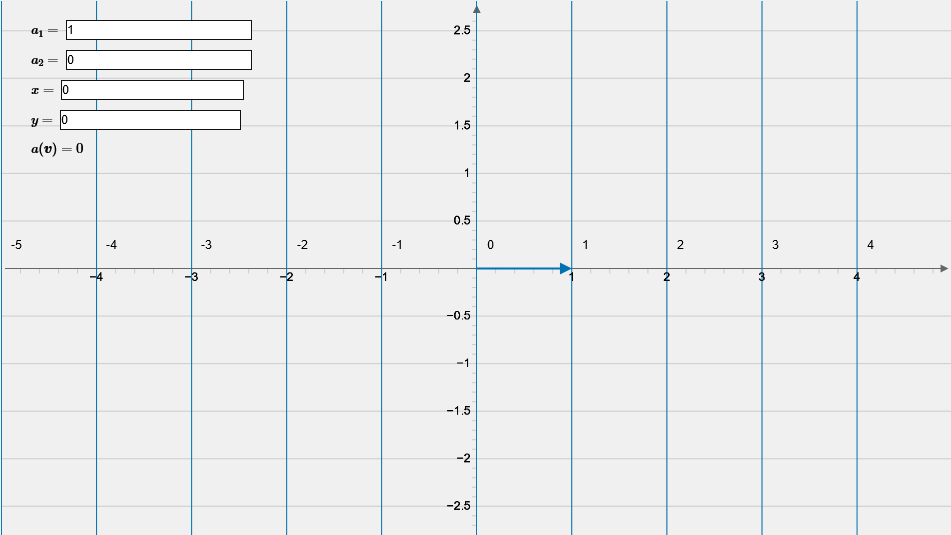
a(n \boldsymbol{b} + m \boldsymbol{c}) = n a(\boldsymbol{b}) + m a(\boldsymbol{c}).

Vectors could be visualized by arrows. Covectors could also be visualized by vectors, but since they are functions, it would not be ideal. A better way is to use curves of constant output value $C$ . Consider a covector with components $a_{\mu}$ and a vector with components $x$ and $y$ :

\begin{align*} \begin{bmatrix}a_1 & a_2\end{bmatrix} \left(\begin{bmatrix} x \\ y \end{bmatrix}\right) &= a_1 x + a_2 y = C, \\ y &= \frac{C - a_1 x}{a_2}, \tag{\(a_2 \neq 0\)} \\ x &= \frac{C - a_2 y}{a_1}, \tag{\(a_1 \neq 0\)} \\ \end{align*}

if we represent the covector as an arrow, it will point perpendicular to the curves and into the direction of increase.

From the applet, we can see that the output can be visualized as the number of lines the vector pierces.

The following holds true for summing covectors:

\begin{align*} (a + b)(\boldsymbol{v}) &= a(\boldsymbol{v}) + b(\boldsymbol{v}), \\ (\begin{bmatrix}a_1 & a_2\end{bmatrix} + \begin{bmatrix}b_1 & b_2\end{bmatrix}) \left(\begin{bmatrix} v^1 \\ v^2 \end{bmatrix}\right) &= (\begin{bmatrix}a_1 + b_1 & a_2 + b_2\end{bmatrix} \left(\begin{bmatrix} v^1 \\ v^2 \end{bmatrix}\right) \\ &= (a_1 + b_1) v^1 + (a_2 + b_2) v^2 \\ &= a_1 v^1 + b_1 v^1 + a_2 v^2 + b_2 v^2 \\ &= a_1 v^1 + a_2 v^2 + b_1 v^1 + b_2 v^2 \\ &= \begin{bmatrix}a_1 & a_2\end{bmatrix} \left(\begin{bmatrix} v^1 \\ v^2 \end{bmatrix}\right) + \begin{bmatrix}b_1 & b_2\end{bmatrix} \left(\begin{bmatrix} v^1 \\ v^2 \end{bmatrix}\right), \end{align*}

and the following for scaling:

\begin{align*} (n a)(\boldsymbol{v}) &= n a(\boldsymbol{v}), \\ (n\begin{bmatrix}a_1 & a_2\end{bmatrix}) \left(\begin{bmatrix} v^1 \\ v^2 \end{bmatrix}\right) &= (\begin{bmatrix}n a_1 & n a_2\end{bmatrix}) \left(\begin{bmatrix} v^1 \\ v^2 \end{bmatrix}\right) \\ &= n a_1 v^1 + n a_2 v^2 \\ &= n (a_1 v^1 + a_2 v^2) \\ &= n \begin{bmatrix}a_1 & a_2\end{bmatrix} \left(\begin{bmatrix} v_1 \\ v_2 \end{bmatrix}\right) \end{align*}

A similar abstract definition can be made: covector is a member of dual vector space $(V^*, S, +, \cdot)$ , where elements of $V^*$ are covectors, $V \to \mathbb{R}$ . Below is a definition of vectors, covectors and their corresponding spaces:

\begin{align*} &\textrm{Vectors are members of vector space \((V, S, +, \cdot)\)} \quad & \quad &\textrm{Covectors are members of dual vector space \((V^*, S, +, \cdot)\)} \\ &\quad V \enspace \textrm{set of vectors} & &\quad V^* \enspace \textrm{set of covectors (functions) - } V \to \mathbb{R} \\ &\quad S \enspace \textrm{set of scalars} & &\quad S \enspace \textrm{set of scalars} \\ &\quad + \enspace (\boldsymbol{v} + \boldsymbol{w})^{\mu} = v^{\mu} + w^{\mu} & &\quad + \enspace (a + b)(\boldsymbol{v}) = a(\boldsymbol{v}) + b(\boldsymbol{v}) \\ &\quad \cdot \enspace (n \boldsymbol{v})^{\mu} = n v^{\mu} & &\quad \cdot \enspace (n a) (\boldsymbol{v}) = n a(\boldsymbol{v}) \\[1.5ex] & & \quad &\textrm{Additional properties (linearity):} \\ & & &\quad a(\boldsymbol{v} + \boldsymbol{w}) = a(\boldsymbol{v}) + a(\boldsymbol{w}) \\ & & &\quad a(n \boldsymbol{v}) = n a(\boldsymbol{v}) \end{align*}

Vectors Are Derivatives

Consider a curve parametrized by $\lambda$ , $\boldsymbol{R}(\lambda)$ :

$Curve$

where the green vector is the tangent vector. In the limiting case when $h \to 0$ :

\lim_{h \to 0} \frac{\boldsymbol{R}(\lambda + h) - \boldsymbol{R}(\lambda)}{h} = \frac{d\boldsymbol{R}}{d\lambda}.

By chain rule, the tangent vector may be written out:

\begin{align*} \frac{d\boldsymbol{R}}{d\lambda} &= \frac{\partial \boldsymbol{R}}{\partial R^{\mu}} \frac{d R^{\mu}}{d \lambda}. \end{align*}

Note: the terms are summed over the $\mu$ components. The term $\frac{d R^{\mu}}{d \lambda}$ makes sense, it's just the derivative of components of $\boldsymbol{R}$ . But the $\frac{\partial \boldsymbol{R}}{\partial R^{\mu}}$ may look a bit weird. To make sense of it, remember that $\boldsymbol{R}$ is the linear combination of the components $R^{\mu}$ and basis vectors $\boldsymbol{e_{\mu}}$ :

\begin{align*} \boldsymbol{R} &= R^{\mu} \boldsymbol{e_{\mu}}, \\ \frac{\partial \boldsymbol{R}}{\partial R^{\mu}} &= \frac{\partial}{\partial R^{\mu}} \left(R^{\mu} \boldsymbol{e_{\mu}}\right) \\ &= \frac{\partial}{\partial R^{\mu}} \left(R^1 \boldsymbol{e_1} + ... + R^{\mu} \boldsymbol{e_{\mu}} + ...\right) \\ &= \frac{\partial}{\partial R^{\mu}} \left(R^1 \boldsymbol{e_1}\right) + ... + \frac{\partial}{\partial R^{\mu}} \left(R^{\mu} \boldsymbol{e_{\mu}}\right) + ... \\ &= 0 + ... + \boldsymbol{e_{\mu}} + ... \\ &= \boldsymbol{e_{\mu}}, \end{align*}

meaning the partial derivative of vector with respect to its component is the basis vector of that component:

\frac{\partial \boldsymbol{R}}{\partial R^{\mu}} = \boldsymbol{e_{\mu}},

however, this definition when we work with intrinsic definitions (if we live on the curve on the image above, we don't have an origin, thus we cannot specify $\boldsymbol{R}$ ), we have to use a different definition:

\frac{\partial}{\partial x^{\mu}} \equiv \boldsymbol{e_{\mu}},

where I replaced $R^{\mu}$ with $x^{\mu}$ . I will sometimes use $\frac{\partial \boldsymbol{R}}{\partial R^{\mu}}$ and sometimes $\frac{\partial}{\partial x^{\mu}}$ . This new definition is on vector space of derivative operators, also called tangent vector space $T_p M$ - vector space of derivatives at point $p$ on the surface $M$ .

Covectors Are Differential Forms

The fact that covectors may be represented by differentials may seem a bit weird initially - how does a covector relate to the differential (e.g. $dx$ ) as are in derivatives and integrals. The multivariable differential is equal to:

df = \frac{\partial f}{\partial x^{\mu}} dx^{\mu},

or in one dimension:

df = \frac{d f}{d x^{\mu}} dx^{\mu}.

We are used that for a variable $x$ , the differential $dx$ means a small change in $x$ . We need to redefine it such that $f$ is a scalar field and $df$ is a covector field.

Consider a function $f(x,y) = x + y$ :

$Plot of f(x,y) = x + y$

The differential $df$ is equal to:

\begin{align*} df &= \frac{\partial f}{\partial x} dx + \frac{\partial f}{\partial y} dy \\ &= dx + dy, \end{align*}

where $dx$ and $dy$ are the dual basis (will be explained later). The covector field may also be written as follows:

df = \begin{bmatrix}1 & 1\end{bmatrix}.

If we input this covector into the applet above, we can visualize the covector field. The lines are the levels of constant $f$ :

$Covector visualization$

The covector $df(\boldsymbol{v})$ is proportional to the steepness of $f$ and to the length of $\boldsymbol{v}$ . From this, we can say that $df(\boldsymbol{v})$ gives us the rate of change of $f$ when moving in the direction of $\boldsymbol{v}$ , which is the directional derivative of $f$ in the direction of $\boldsymbol{v}$ :

df(\boldsymbol{v}) = \nabla_{\boldsymbol{v}} f = \frac{\partial f}{\partial \boldsymbol{v}}.

Consider covector field $df$ acts on the basis vectors $\frac{\partial}{\partial x}$ and $\frac{\partial}{\partial y}$ :

\begin{align*} df \left(\frac{\partial}{\partial x}\right) &= \frac{\partial f}{\partial x}, \tag{directional derivative of \(f\) in the \(x\) direction} \\ df \left(\frac{\partial}{\partial y}\right) &= \frac{\partial f}{\partial y}. \tag{directional derivative of \(f\) in the \(y\) direction} \\ \end{align*}

Now, consider the scalar field $x$ , where the value is just the value of $x$ at the point:

$Plot of x$

the covector field $dx$ looks like this:

$Plot of dx$

and the covector field $dx$ acts on the basis vectors $\frac{\partial}{\partial x}$ and $\frac{\partial}{\partial y}$ as follows:

\begin{align*} dx \left(\frac{\partial}{\partial x}\right) &= \frac{\partial x}{\partial x} = 1, \tag{directional derivative of \(x\) in the \(x\) direction} \\ dx \left(\frac{\partial}{\partial y}\right) &= \frac{\partial x}{\partial y} = 0. \tag{directional derivative of \(x\) in the \(y\) direction} \\ \end{align*}

Similarly, the covector field $dy$ acts on the basis vectors $\frac{\partial}{\partial x}$ and $\frac{\partial}{\partial y}$ as follows:

\begin{align*} dy \left(\frac{\partial}{\partial x}\right) &= \frac{\partial y}{\partial x} = 0, \tag{directional derivative of \(y\) in the \(x\) direction} \\ dy \left(\frac{\partial}{\partial y}\right) &= \frac{\partial y}{\partial y} = 1. \tag{directional derivative of \(y\) in the \(y\) direction} \\ \end{align*}

So we introduce special covectors $\epsilon^{\mu}$ called the dual basis, such that:

\epsilon^{\mu} (\boldsymbol{e_{\nu}}) = \delta^{\mu}_{\nu},

where $\delta^{\mu}_{\nu}$ is the Kronecker delta:

\delta^{\mu}_{\nu} = \begin{cases} 1 & \mu &= \nu, \\ 0 & \mu &\neq \nu. \end{cases}

Which is identical to the previous equations with differentials and derivatives:

dx^{\mu} \left(\frac{\partial}{\partial x^{\nu}}\right) = \frac{\partial x^{\mu}}{\partial x^{\nu}} = \delta^{\mu}_{\nu}.

The derivative of $f$ with respect to $\lambda$ may be rewritten as the covector $df$ acting on the vector $\frac{d}{d \lambda}$ :

\frac{df}{d\lambda} = df \left(\frac{d}{d \lambda}\right).