Back Interpretation of the Schwarzschild Coordinates The metric is in the form:
d s 2 = − ( 1 − 2 r ) d t 2 + ( 1 − 2 r ) − 1 d r 2 + r 2 d ϕ 2 . ds^2 = -\left(1 - \frac{2}{r}\right) dt^2 + \left(1 - \frac{2}{r}\right)^{-1} dr^2 + r^2 d\phi^2. d s 2 = − ( 1 − r 2 ) d t 2 + ( 1 − r 2 ) − 1 d r 2 + r 2 d ϕ 2 . For constant ( r , θ , ϕ ) (r, \theta, \phi) ( r , θ , ϕ )
d s 2 = − ( 1 − 2 r ) d t 2 . ds^2 = -\left(1 - \frac{2}{r}\right) dt^2. d s 2 = − ( 1 − r 2 ) d t 2 . For timelike paths, this is equal to the negative proper time τ \tau τ
− d τ 2 = − ( 1 − 2 r ) d t 2 , d τ 2 = ( 1 − 2 r ) d t 2 , d τ = 1 − 2 r d t , ∫ 0 τ d τ = 1 − 2 r ∫ 0 t d t , τ = 1 − 2 r t . \begin{align*} -d\tau^2 &= -\left(1 - \frac{2}{r}\right) dt^2, \\ d\tau^2 &= \left(1 - \frac{2}{r}\right) dt^2, \\ d\tau &= \sqrt{1 - \frac{2}{r}} dt, \\ \int_0^{\tau} d\tau &= \sqrt{1 - \frac{2}{r}} \int_0^t dt, \\ \tau &= \sqrt{1 - \frac{2}{r}} t. \\ \end{align*} − d τ 2 d τ 2 d τ ∫ 0 τ d τ τ = − ( 1 − r 2 ) d t 2 , = ( 1 − r 2 ) d t 2 , = 1 − r 2 d t , = 1 − r 2 ∫ 0 t d t , = 1 − r 2 t . Below is a table evaluating the time dilation at different r r r
r \boldsymbol{r} r τ \boldsymbol{\tau} τ r s r_s r s 0 0 0 2 r s 2r_s 2 r s ≈ 0.71 t \approx 0.71t ≈ 0.71 t ∞ \infty ∞ t t t
For proper length, we will take t , θ , ϕ t, \theta, \phi t , θ , ϕ
d s 2 = ( 1 − 2 r ) − 1 d r 2 . ds^2 = \left(1 - \frac{2}{r}\right)^{-1} dr^2. d s 2 = ( 1 − r 2 ) − 1 d r 2 . For spacelike paths, this is equal to the proper length:
d L 0 2 = ( r − 2 r ) − 1 d r 2 , d L 0 = r r − 2 d r , ∫ 0 L 0 d L 0 = ∫ r 0 r r r − 2 d r , L 0 = ∫ r 0 r r r − 2 d r , r = u 2 , d r = 2 u d u , u = r , L 0 = ∫ r 0 r u 2 u 2 − 2 2 u d u = 2 ∫ r 0 r u 2 u 2 − 2 d u , u = 2 y , d u = 2 d y , y = u 2 , L 0 = 2 ∫ r 0 2 r 2 2 y 2 2 y 2 − 2 2 d y = 4 ∫ r 0 2 r 2 y 2 2 y 2 − 1 2 d y = 4 ∫ r 0 2 r 2 y 2 y 2 − 1 d y , y = cosh α , d y = sinh α d α , α = cosh − 1 y , L 0 = 4 ∫ cosh − 1 r 0 2 cosh − 1 r 2 cosh 2 α cosh 2 α − 1 sinh α d α = 4 ∫ cosh − 1 r 0 2 cosh − 1 r 2 cosh 2 α d α = 4 ∫ cosh − 1 r 0 2 cosh − 1 r 2 cosh 2 α + 1 2 d α = ∫ cosh − 1 r 0 2 cosh − 1 r 2 2 ( cosh 2 α + 1 ) d α , β = 2 α , d β = 2 d α , L 0 = ∫ 2 cosh − 1 r 0 2 2 cosh − 1 r 2 ( cosh β + 1 ) d β = [ sinh β + β ] 2 cosh − 1 r 0 2 2 cosh − 1 r 2 . \begin{align*} dL_0{}^2 &= \left(\frac{r - 2}{r}\right)^{-1} dr^2, \\ dL_0 &= \sqrt{\frac{r}{r - 2}} dr, \\ \int_0^{L_0} dL_0 &= \int_{r_0}^r \sqrt{\frac{r}{r - 2}} dr, \\ L_0 &= \int_{r_0}^r \sqrt{\frac{r}{r - 2}} dr, \\ r &= u^2, \\ dr &= 2u\ du, \\ u &= \sqrt{r}, \\ L_0 &= \int_{\sqrt{r_0}}^{\sqrt{r}} \sqrt{\frac{u^2}{u^2 - 2}} 2u\ du \\ &= 2 \int_{\sqrt{r_0}}^{\sqrt{r}} \frac{u^2}{\sqrt{u^2 - 2}} du, \\ u &= \sqrt{2} y, \\ du &= \sqrt{2}\ dy, \\ y &= \frac{u}{\sqrt{2}}, \\ L_0 &= 2 \int_{\sqrt{\frac{r_0}{2}}}^{\sqrt{\frac{r}{2}}} \frac{2y^2}{\sqrt{2y^2 - 2}} \sqrt{2}\ dy \\ &= 4 \int_{\sqrt{\frac{r_0}{2}}}^{\sqrt{\frac{r}{2}}} \frac{y^2}{\sqrt{2} \sqrt{y^2 - 1}} \sqrt{2}\ dy \\ &= 4 \int_{\sqrt{\frac{r_0}{2}}}^{\sqrt{\frac{r}{2}}} \frac{y^2}{\sqrt{y^2 - 1}} dy, \\ y &= \cosh \alpha, \\ dy &= \sinh \alpha\ d\alpha, \\ \alpha &= \cosh^{-1} y, \\ L_0 &= 4 \int_{\cosh^{-1} \sqrt{\frac{r_0}{2}}}^{\cosh^{-1} \sqrt{\frac{r}{2}}} \frac{\cosh^2 {\alpha}}{\sqrt{\cosh^2 \alpha - 1}} \sinh \alpha\ d\alpha \\ &= 4 \int_{\cosh^{-1} \sqrt{\frac{r_0}{2}}}^{\cosh^{-1} \sqrt{\frac{r}{2}}} \cosh^2 {\alpha}\ d\alpha \\ &= 4 \int_{\cosh^{-1} \sqrt{\frac{r_0}{2}}}^{\cosh^{-1} \sqrt{\frac{r}{2}}} \frac{\cosh 2\alpha + 1}{2} d\alpha \\ &= \int_{\cosh^{-1} \sqrt{\frac{r_0}{2}}}^{\cosh^{-1} \sqrt{\frac{r}{2}}} 2 (\cosh 2\alpha + 1)\ d\alpha, \\ \beta &= 2 \alpha, \\ d\beta &= 2\ d\alpha, \\ L_0 &= \int_{2\cosh^{-1} \sqrt{\frac{r_0}{2}}}^{2\cosh^{-1} \sqrt{\frac{r}{2}}} (\cosh \beta + 1)\ d\beta \\ &= \left[\sinh \beta + \beta\right]_{2\cosh^{-1} \sqrt{\frac{r_0}{2}}}^{2\cosh^{-1} \sqrt{\frac{r}{2}}}. \\ \end{align*} d L 0 2 d L 0 ∫ 0 L 0 d L 0 L 0 r d r u L 0 u d u y L 0 y d y α L 0 β d β L 0 = ( r r − 2 ) − 1 d r 2 , = r − 2 r d r , = ∫ r 0 r r − 2 r d r , = ∫ r 0 r r − 2 r d r , = u 2 , = 2 u d u , = r , = ∫ r 0 r u 2 − 2 u 2 2 u d u = 2 ∫ r 0 r u 2 − 2 u 2 d u , = 2 y , = 2 d y , = 2 u , = 2 ∫ 2 r 0 2 r 2 y 2 − 2 2 y 2 2 d y = 4 ∫ 2 r 0 2 r 2 y 2 − 1 y 2 2 d y = 4 ∫ 2 r 0 2 r y 2 − 1 y 2 d y , = cosh α , = sinh α d α , = cosh − 1 y , = 4 ∫ c o s h − 1 2 r 0 c o s h − 1 2 r cosh 2 α − 1 cosh 2 α sinh α d α = 4 ∫ c o s h − 1 2 r 0 c o s h − 1 2 r cosh 2 α d α = 4 ∫ c o s h − 1 2 r 0 c o s h − 1 2 r 2 cosh 2 α + 1 d α = ∫ c o s h − 1 2 r 0 c o s h − 1 2 r 2 ( cosh 2 α + 1 ) d α , = 2 α , = 2 d α , = ∫ 2 c o s h − 1 2 r 0 2 c o s h − 1 2 r ( cosh β + 1 ) d β = [ sinh β + β ] 2 c o s h − 1 2 r 0 2 c o s h − 1 2 r . The magnitude of r r r
The function is approximately linear at a distance further away from the object.
For the proper length of circumference, we will take t , r , θ t, r, \theta t , r , θ
d s 2 = r 2 d ϕ 2 . ds^2 = r^2 d\phi^2. d s 2 = r 2 d ϕ 2 . As for the radius, this is equal to the proper length:
d L 0 2 = r 2 d ϕ 2 , d L 0 = r d ϕ , ∫ 0 L 0 d L 0 = r ∫ 0 2 π d ϕ , L 0 = 2 π r . \begin{align*} dL_0{}^2 &= r^2 d\phi^2, \\ dL_0 &= r d\phi, \\ \int_0^{L_0} dL_0 &= r \int_{0}^{2 \pi} d\phi, \\ L_0 &= 2 \pi r. \end{align*} d L 0 2 d L 0 ∫ 0 L 0 d L 0 L 0 = r 2 d ϕ 2 , = r d ϕ , = r ∫ 0 2 π d ϕ , = 2 π r . The r r r
We will take constant t , θ t, \theta t , θ
d s 2 = ( 1 − 2 r ) − 1 d r 2 + r 2 d ϕ 2 . ds^2 = \left(1 - \frac{2}{r}\right)^{-1} dr^2 + r^2 d\phi^2. d s 2 = ( 1 − r 2 ) − 1 d r 2 + r 2 d ϕ 2 . We will begin by considering the cylindrical coordinates:
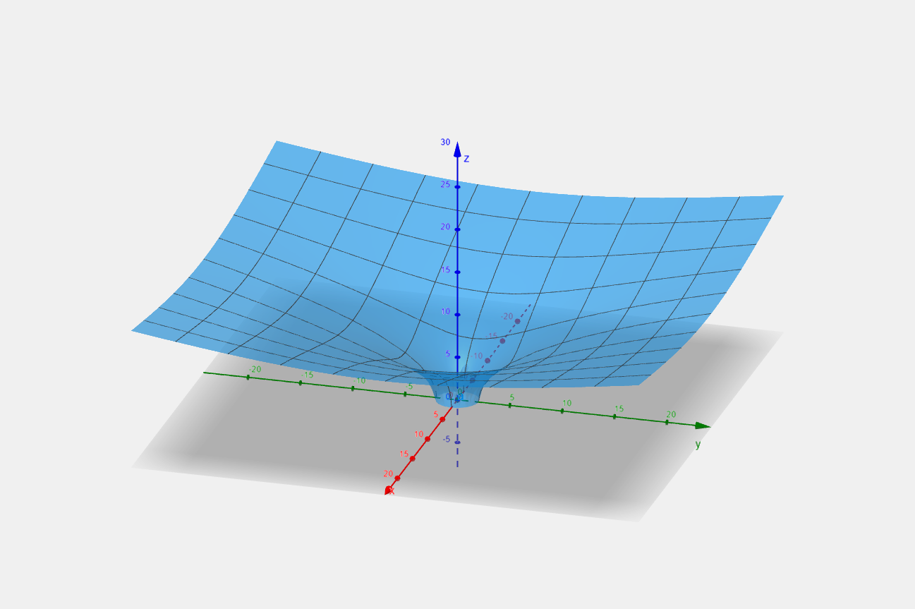
d s 2 = d r 2 + r 2 d ϕ 2 + d z 2 , d s 2 = ( ( d z d r ) 2 + 1 ) d r 2 + r 2 d ϕ 2 , \begin{align*} ds^2 &= dr^2 + r^2 d\phi^2 + dz^2, \\ ds^2 &= \left(\left(\frac{dz}{dr}\right)^2 + 1\right) dr^2 + r^2 d\phi^2, \end{align*} d s 2 d s 2 = d r 2 + r 2 d ϕ 2 + d z 2 , = ( ( d r d z ) 2 + 1 ) d r 2 + r 2 d ϕ 2 , and make the line elements equal and solve for z z z
( 1 − 2 r ) − 1 d r 2 + r 2 d ϕ 2 = ( ( d z d r ) 2 + 1 ) d r 2 + r 2 d ϕ 2 , ( r − 2 r ) − 1 d r 2 = ( ( d z d r ) 2 + 1 ) d r 2 , ( d z d r ) 2 + 1 = r r − 2 , ( d z d r ) 2 = r r − 2 − 1 = 2 r − 2 , d z d r = 2 r − 2 , ∫ z 0 z d z = ∫ r 0 r 2 r − 2 d r , z − z 0 = 2 2 [ r − 2 ] r 0 r , z = 2 2 [ r − 2 ] r 0 r + z 0 , \begin{align*} \left(1 - \frac{2}{r}\right)^{-1} dr^2 + r^2 d\phi^2 &= \left(\left(\frac{dz}{dr}\right)^2 + 1\right) dr^2 + r^2 d\phi^2, \\ \left(\frac{r - 2}{r}\right)^{-1} dr^2 &= \left(\left(\frac{dz}{dr}\right)^2 + 1\right) dr^2, \\ \left(\frac{dz}{dr}\right)^2 + 1 &= \frac{r}{r - 2}, \\ \left(\frac{dz}{dr}\right)^2 &= \frac{r}{r - 2} - 1 \\ &= \frac{2}{r - 2}, \\ \frac{dz}{dr} &= \sqrt{\frac{2}{r - 2}}, \\ \int_{z_0}^z dz &= \int_{r_0}^r \sqrt{\frac{2}{r - 2}} dr, \\ z - z_0 &= 2 \sqrt{2} [\sqrt{r - 2}]_{r_0}^r, \\ z &= 2 \sqrt{2} [\sqrt{r - 2}]_{r_0}^r + z_0, \\ \end{align*} ( 1 − r 2 ) − 1 d r 2 + r 2 d ϕ 2 ( r r − 2 ) − 1 d r 2 ( d r d z ) 2 + 1 ( d r d z ) 2 d r d z ∫ z 0 z d z z − z 0 z = ( ( d r d z ) 2 + 1 ) d r 2 + r 2 d ϕ 2 , = ( ( d r d z ) 2 + 1 ) d r 2 , = r − 2 r , = r − 2 r − 1 = r − 2 2 , = r − 2 2 , = ∫ r 0 r r − 2 2 d r , = 2 2 [ r − 2 ] r 0 r , = 2 2 [ r − 2 ] r 0 r + z 0 , where z 0 z_0 z 0 z z z r = r 0 r = r_0 r = r 0
here, r 0 = 2 r_0 = 2 r 0 = 2 z 0 = 0 z_0 = 0 z 0 = 0
There are two singularities. The first one is in the g 11 g_{11} g 11 r → r s + r \to r_s^+ r → r s +
lim r → r s + g 11 = lim r → 2 + ( 1 − 2 r ) − 1 = lim r → 2 + r r − 2 = ∞ , \begin{align*} \lim_{r \to r_s^+} g_{11} &= \lim_{r \to 2^+} \left(1 - \frac{2}{r}\right)^{-1} \\ &= \lim_{r \to 2^+} \frac{r}{r - 2} = \infty, \end{align*} r → r s + lim g 11 = r → 2 + lim ( 1 − r 2 ) − 1 = r → 2 + lim r − 2 r = ∞ , this is a coordinate singularity. We can get rid of it by changing coordinates. The other singularity is in the g 00 g_{00} g 00 r → 0 + r \to 0^+ r → 0 +
lim r → 0 + g 00 = lim r → 0 + − ( 1 − 2 r ) = lim r → 0 + 2 − r r = ∞ , \begin{align*} \lim_{r \to 0^+} g_{00} &= \lim_{r \to 0^+} - \left(1 - \frac{2}{r}\right) \\ &= \lim_{r \to 0^+} \frac{2 - r}{r} = \infty, \end{align*} r → 0 + lim g 00 = r → 0 + lim − ( 1 − r 2 ) = r → 0 + lim r 2 − r = ∞ , this, unfortunately, is a true singularity and at this point general relativity stops making sense.