Back Gauss's Law By Gauss's Law, the electric flux through a closed surface is equal to the total charge enclosed within that surface divided by the permittivity:
Φ E = ∯ S E ⋅ d A = Q ϵ 0 , I n t e g r a l f o r m ∇ ⋅ E = ρ ϵ 0 ϵ r , D i f f e r e n t i a l f o r m \begin{align*} \Phi_E &= \oiint_S \boldsymbol{E} \cdot d \boldsymbol{A} = \frac{Q}{\epsilon_0}, & &\mathrm{Integral\ form}\\ \boldsymbol{\nabla} \cdot \boldsymbol{E} &= \frac{\rho}{\epsilon_0 \epsilon_r}, & &\mathrm{Differential\ form} \end{align*} Φ E ∇ ⋅ E = ∬ S E ⋅ d A = ϵ 0 Q , = ϵ 0 ϵ r ρ , Integral form Differential form where:
ϵ 0 ≈ 8.85 ⋅ 1 0 − 12 F m − 1 , k e = 1 4 π ϵ 0 ⟹ ϵ 0 = 1 4 π k e , \begin{align*} \epsilon_0 &\approx 8.85 \cdot 10^{-12}\ Fm^{-1}, \\ k_e &= \frac{1}{4 \pi \epsilon_0} \implies \epsilon_0 = \frac{1}{4 \pi k_e}, \end{align*} ϵ 0 k e ≈ 8.85 ⋅ 1 0 − 12 F m − 1 , = 4 π ϵ 0 1 ⟹ ϵ 0 = 4 π k e 1 , and where A A A
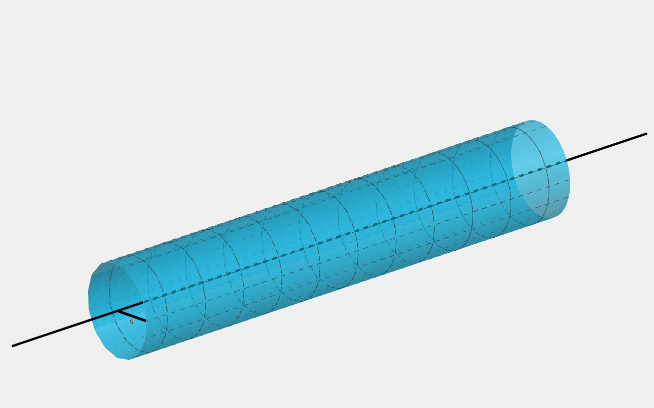
A line has a constant linear charge density λ \lambda λ A A A B B B C C C
This example builds on the linear algebra of line charge from electric field , particularly:
h y = y ^ ⋅ ( C − A ) , h = h y y ^ , H = A + h , s = C − H . \begin{align*} h_y &= \boldsymbol{\hat{y}} \cdot (C - A), \\ \boldsymbol{h} &= h_y \boldsymbol{\hat{y}}, \\ H &= A + \boldsymbol{h}, \\ \boldsymbol{s} &= C - H. \end{align*} h y h H s = y ^ ⋅ ( C − A ) , = h y y ^ , = A + h , = C − H . Since the charge density λ \lambda λ
Then the electric flux is equal to:
Φ E = ∯ S E ⋅ d A = λ l ϵ 0 \Phi_E = \oiint_S \boldsymbol{E} \cdot d \boldsymbol{A} = \frac{\lambda l}{\epsilon_0} Φ E = ∬ S E ⋅ d A = ϵ 0 λ l The electric field's direction and magnitude does not depend on A A A
E A = λ l ϵ 0 , 2 E π s l = λ l ϵ 0 , E = λ 2 π s 1 4 π k e = λ s 1 2 k e = 2 k e λ s , \begin{align*} E A &= \frac{\lambda l}{\epsilon_0}, \\ 2 E \pi s l &= \frac{\lambda l}{\epsilon_0}, \\ E &= \frac{\lambda}{2 \pi s \frac{1}{4 \pi k_e}} \\ &= \frac{\lambda}{s \frac{1}{2 k_e}} \\ &= \frac{2 k_e \lambda}{s}, \\ \end{align*} E A 2 E π s l E = ϵ 0 λ l , = ϵ 0 λ l , = 2 π s 4 π k e 1 λ = s 2 k e 1 λ = s 2 k e λ , The vector is pointing in the direction perpendicular to the line. This is identical to the equation derived in the electric field section with the infinite line charge .
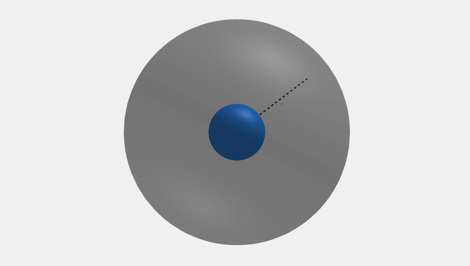
A spherical conductor of radius r c r_c r c constant surface area charge density σ \sigma σ r r r
The charge density σ \sigma σ
Q = σ S , = 4 σ π r c 2 . \begin{align*} Q &= \sigma S, \\ &= 4 \sigma \pi r_c^2. \end{align*} Q = σ S , = 4 σπ r c 2 . The electric flux is equal to:
Φ E = ∯ S E ⋅ d A = 4 σ π r c 2 ϵ 0 \Phi_E = \oiint_S \boldsymbol{E} \cdot d \boldsymbol{A} = \frac{4 \sigma \pi r_c^2}{\epsilon_0} Φ E = ∬ S E ⋅ d A = ϵ 0 4 σπ r c 2 Similar to previous scenario , the electric field does not depend on A A A
E A = 4 σ π r c 2 ϵ 0 , 4 E π r 2 = 4 σ π r c 2 ϵ 0 , E = r c 2 σ r 2 ϵ 0 , \begin{align*} E A &= \frac{4 \sigma \pi r_c^2}{\epsilon_0}, \\ 4 E \pi r^2 &= \frac{4 \sigma \pi r_c^2}{\epsilon_0}, \\ E &= \frac{r_c^2 \sigma}{r^2 \epsilon_0}, \\ \end{align*} E A 4 E π r 2 E = ϵ 0 4 σπ r c 2 , = ϵ 0 4 σπ r c 2 , = r 2 ϵ 0 r c 2 σ ,
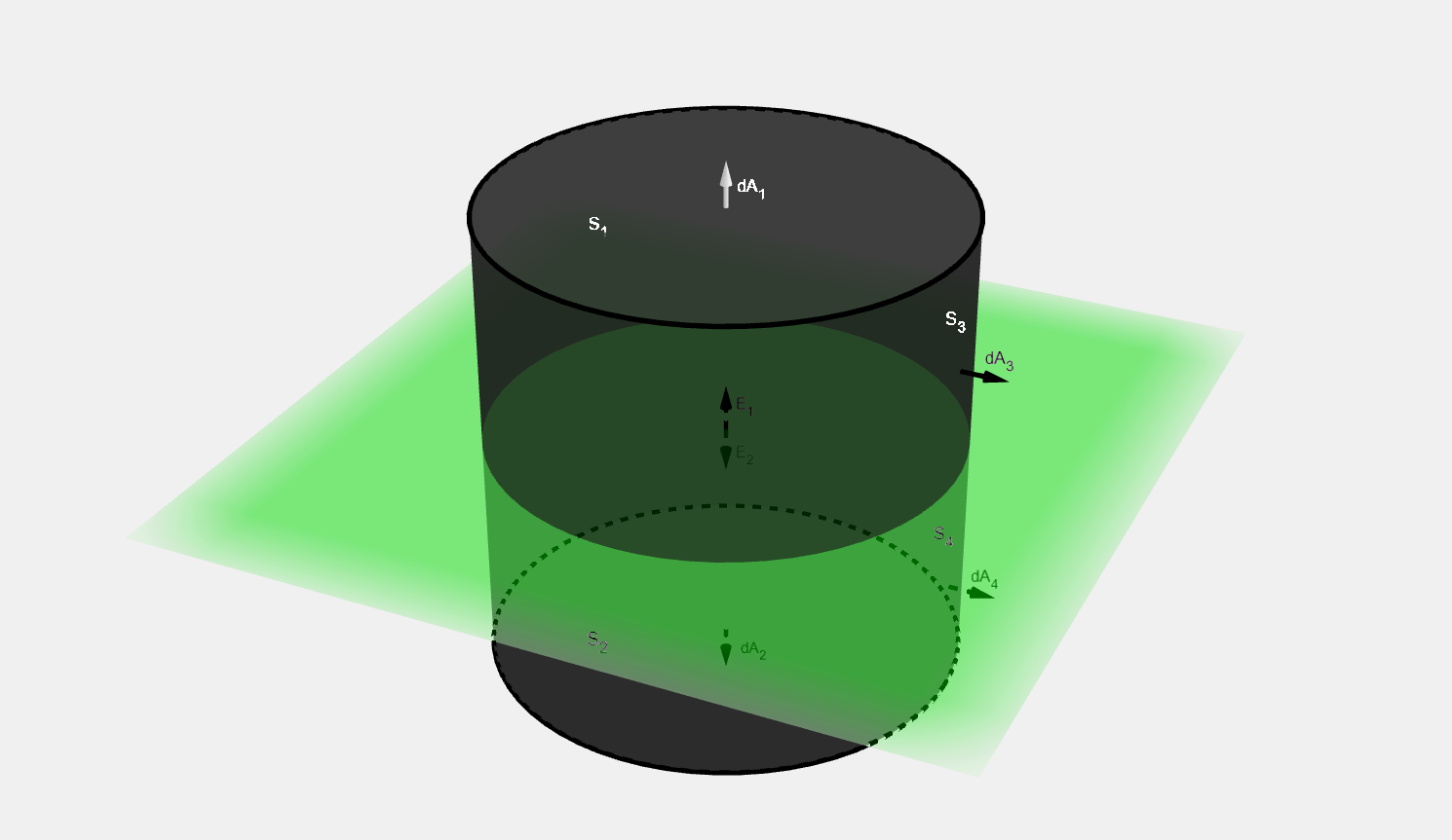
A plane has a uniform charge density σ \sigma σ
The plane divides the space into two sectors, z < 0 z < 0 z < 0 z > 0 z > 0 z > 0 E 1 = − E 2 \boldsymbol{E_1} = -\boldsymbol{E_2} E 1 = − E 2
We construct a cylinder:
Where A = A 1 = A 2 A = A_1 = A_2 A = A 1 = A 2
Then the total electric flux is equal to:
Φ E = ∯ S E ⋅ d A = ∬ S 1 E 1 ⋅ d A 1 + ∬ S 2 E 2 ⋅ d A 2 + ∬ S 3 E 3 ⋅ d A 3 + ∬ S 4 E 4 ⋅ d A 4 = E 1 A 1 + E 2 A 2 = 2 E A . \begin{align*} \Phi_E &= \oiint_S \boldsymbol{E} \cdot d\boldsymbol{A} \\ &= \iint_{S_1} \boldsymbol{E_1} \cdot d\boldsymbol{A_1} + \iint_{S_2} \boldsymbol{E_2} \cdot d\boldsymbol{A_2} + \iint_{S_3} \boldsymbol{E_3} \cdot d\boldsymbol{A_3} + \iint_{S_4} \boldsymbol{E_4} \cdot d\boldsymbol{A_4} \\ &= E_1 A_1 + E_2 A_2 \\ &= 2 E A. \end{align*} Φ E = ∬ S E ⋅ d A = ∬ S 1 E 1 ⋅ d A 1 + ∬ S 2 E 2 ⋅ d A 2 + ∬ S 3 E 3 ⋅ d A 3 + ∬ S 4 E 4 ⋅ d A 4 = E 1 A 1 + E 2 A 2 = 2 E A . Since the charge density is constant, the total charge is equal to:
Using Gauss's law:
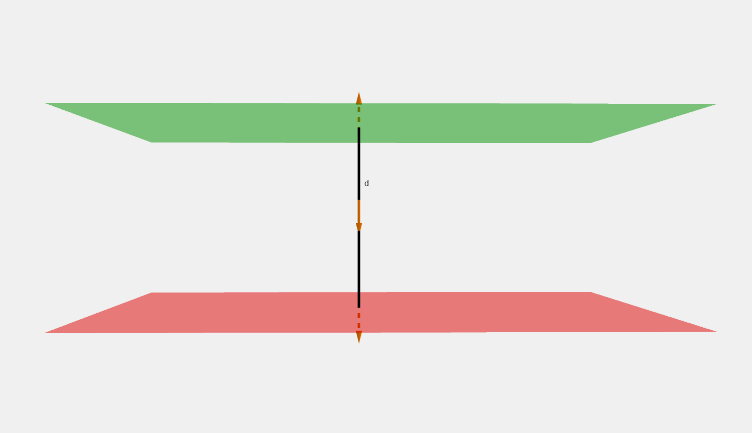
2 E A = σ A ϵ 0 , E = σ 2 ϵ 0 , E = { σ 2 ϵ 0 z ^ z > 0 , − σ 2 ϵ 0 z ^ z < 0. \begin{align*} 2 E A &= \frac{\sigma A}{\epsilon_0}, \\ E &= \frac{\sigma}{2 \epsilon_0}, \\ \boldsymbol{E} &= \begin{cases} \ \ \ \frac{\sigma}{2 \epsilon_0}\boldsymbol{\hat{z}} & z > 0, \\ -\frac{\sigma}{2 \epsilon_0}\boldsymbol{\hat{z}} & z < 0. \end{cases} \end{align*} 2 E A E E = ϵ 0 σ A , = 2 ϵ 0 σ , = { 2 ϵ 0 σ z ^ − 2 ϵ 0 σ z ^ z > 0 , z < 0. Two parallel infinite planes at a distance d d d σ \sigma σ
The electric field is the sum of electric fields caused by each plane:
E = E + + E − , E + = { σ 2 ϵ 0 z ^ z > d 2 , − σ 2 ϵ 0 z ^ z < d 2 , E − = { − σ 2 ϵ 0 z ^ z > − d 2 , σ 2 ϵ 0 z ^ z < − d 2 , E = { 0 z > d 2 or z < − d 2 , − σ ϵ 0 z ^ − d 2 < z < d 2 . \begin{align*} \boldsymbol{E} &= \boldsymbol{E_+} + \boldsymbol{E_-}, \\ \boldsymbol{E_+} &= \begin{cases} \ \ \ \frac{\sigma}{2 \epsilon_0}\boldsymbol{\hat{z}} & z > \frac{d}{2}, \\ -\frac{\sigma}{2 \epsilon_0}\boldsymbol{\hat{z}} & z < \frac{d}{2}, \end{cases} \\ \boldsymbol{E_-} &= \begin{cases} -\frac{\sigma}{2 \epsilon_0}\boldsymbol{\hat{z}} & z > -\frac{d}{2}, \\ \ \ \ \frac{\sigma}{2 \epsilon_0}\boldsymbol{\hat{z}} & z < -\frac{d}{2}, \end{cases} \\ \boldsymbol{E} &= \begin{cases} \ \ \ \boldsymbol{0} & \ \ \ z > \frac{d}{2}\ \textrm{or}\ z < -\frac{d}{2}, \\ -\frac{\sigma}{\epsilon_0}\boldsymbol{\hat{z}} & -\frac{d}{2} < z < \frac{d}{2}. \end{cases} \end{align*} E E + E − E = E + + E − , = { 2 ϵ 0 σ z ^ − 2 ϵ 0 σ z ^ z > 2 d , z < 2 d , = { − 2 ϵ 0 σ z ^ 2 ϵ 0 σ z ^ z > − 2 d , z < − 2 d , = { 0 − ϵ 0 σ z ^ z > 2 d or z < − 2 d , − 2 d < z < 2 d .