Back Ricci Tensor and Ricci Scalar Ricci tensor tracks how volume changes along geodesics. We can say it "summarizes" the Riemann tensor. Ricci scalar tells us how a volume is different than in flat space.
Recall the geodesic deviation from the previous chapter :
∇ v ∇ v s = − R ( s , v ) v . \nabla_{\boldsymbol{v}} \nabla_{\boldsymbol{v}} \boldsymbol{s} = -R(\boldsymbol{s}, \boldsymbol{v}) \boldsymbol{v}. ∇ v ∇ v s = − R ( s , v ) v . Flat space
Curved space
Curved space
[ R ( s , v ) v ] ⋅ s = 0 [R(\boldsymbol{s}, \boldsymbol{v}) \boldsymbol{v}] \cdot \boldsymbol{s} = 0 [ R ( s , v ) v ] ⋅ s = 0 [ R ( s , v ) v ] ⋅ s > 0 [R(\boldsymbol{s}, \boldsymbol{v}) \boldsymbol{v}] \cdot \boldsymbol{s} > 0 [ R ( s , v ) v ] ⋅ s > 0 [ R ( s , v ) v ] ⋅ s < 0 [R(\boldsymbol{s}, \boldsymbol{v}) \boldsymbol{v}] \cdot \boldsymbol{s} < 0 [ R ( s , v ) v ] ⋅ s < 0 The dot product of Riemann tensor and the separation vector depends on the sizes of v \boldsymbol{v} v s \boldsymbol{s} s
[ R ( s , v ) v ] ⋅ s ∣ s × v ∣ 2 = [ R ( s , v ) v ] ⋅ s ∣ s ∣ 2 ∣ v ∣ 2 sin 2 θ = [ R ( s , v ) v ] ⋅ s ∣ s ∣ 2 ∣ v ∣ 2 sin 2 θ = [ R ( s , v ) v ] ⋅ s ∣ s ∣ 2 ∣ v ∣ 2 ( 1 − cos 2 θ ) = [ R ( s , v ) v ] ⋅ s ∣ s ∣ 2 ∣ v ∣ 2 − ( ∣ s ∣ ∣ v ∣ cos θ ) 2 = [ R ( s , v ) v ] ⋅ s ( s ⋅ s ) ( v ⋅ v ) − ( s ⋅ v ) . \begin{align*} \frac{[R(\boldsymbol{s}, \boldsymbol{v}) \boldsymbol{v}] \cdot \boldsymbol{s}}{|\boldsymbol{s} \times \boldsymbol{v}|^2} &= \frac{[R(\boldsymbol{s}, \boldsymbol{v}) \boldsymbol{v}] \cdot \boldsymbol{s}}{|\boldsymbol{s}|^2 |\boldsymbol{v}|^2 \sin^2 \theta} \\ &= \frac{[R(\boldsymbol{s}, \boldsymbol{v}) \boldsymbol{v}] \cdot \boldsymbol{s}}{|\boldsymbol{s}|^2 |\boldsymbol{v}|^2 \sin^2 \theta} \\ &= \frac{[R(\boldsymbol{s}, \boldsymbol{v}) \boldsymbol{v}] \cdot \boldsymbol{s}}{|\boldsymbol{s}|^2 |\boldsymbol{v}|^2 (1 - \cos^2 \theta)} \\ &= \frac{[R(\boldsymbol{s}, \boldsymbol{v}) \boldsymbol{v}] \cdot \boldsymbol{s}}{|\boldsymbol{s}|^2 |\boldsymbol{v}|^2 - (|\boldsymbol{s}| |\boldsymbol{v}| \cos \theta)^2} \\ &= \frac{[R(\boldsymbol{s}, \boldsymbol{v}) \boldsymbol{v}] \cdot \boldsymbol{s}}{(\boldsymbol{s} \cdot \boldsymbol{s}) (\boldsymbol{v} \cdot \boldsymbol{v}) - (\boldsymbol{s} \cdot \boldsymbol{v})}. \end{align*} ∣ s × v ∣ 2 [ R ( s , v ) v ] ⋅ s = ∣ s ∣ 2 ∣ v ∣ 2 sin 2 θ [ R ( s , v ) v ] ⋅ s = ∣ s ∣ 2 ∣ v ∣ 2 sin 2 θ [ R ( s , v ) v ] ⋅ s = ∣ s ∣ 2 ∣ v ∣ 2 ( 1 − cos 2 θ ) [ R ( s , v ) v ] ⋅ s = ∣ s ∣ 2 ∣ v ∣ 2 − ( ∣ s ∣∣ v ∣ cos θ ) 2 [ R ( s , v ) v ] ⋅ s = ( s ⋅ s ) ( v ⋅ v ) − ( s ⋅ v ) [ R ( s , v ) v ] ⋅ s . We can prove the formula stays constant by transforming s → a s + b v \boldsymbol{s} \to a\boldsymbol{s} + b\boldsymbol{v} s → a s + b v v → c s + d v \boldsymbol{v} \to c\boldsymbol{s} + d\boldsymbol{v} v → c s + d v
R ( a s + b v , c s + d v ) = R ( a s , c s + d v ) + R ( b v , c s + d v ) = a c R ( s , s ) + a d R ( s , v ) + b c R ( v , s ) + b d R ( v , v ) = a d R ( s , v ) − b c R ( s , v ) = ( a d − b c ) R ( s , v ) . \begin{align*} R(a\boldsymbol{s} + b\boldsymbol{v}, c\boldsymbol{s} + d\boldsymbol{v}) &= R(a\boldsymbol{s}, c\boldsymbol{s} + d\boldsymbol{v}) + R(b\boldsymbol{v}, c\boldsymbol{s} + d\boldsymbol{v}) \\ &= ac R(\boldsymbol{s}, \boldsymbol{s}) + ad R(\boldsymbol{s}, \boldsymbol{v}) \\ &+ bc R(\boldsymbol{v}, \boldsymbol{s}) + bd R(\boldsymbol{v}, \boldsymbol{v}) \\ &= ad R(\boldsymbol{s}, \boldsymbol{v}) - bc R(\boldsymbol{s}, \boldsymbol{v}) \\ &= (ad - bc) R(\boldsymbol{s}, \boldsymbol{v}). \end{align*} R ( a s + b v , c s + d v ) = R ( a s , c s + d v ) + R ( b v , c s + d v ) = a c R ( s , s ) + a d R ( s , v ) + b c R ( v , s ) + b d R ( v , v ) = a d R ( s , v ) − b c R ( s , v ) = ( a d − b c ) R ( s , v ) . Recall that the Riemann tensor acting on a dot product is zero:
R ( e α , e β ) ( a ⋅ b ) = R ( e α , e β ) a ⋅ b + a ⋅ R ( e α , e β ) b = 0 , R ( e α , e β ) a ⋅ b = − a ⋅ R ( e α , e β ) b , \begin{align*} R(\boldsymbol{e_{\alpha}}, \boldsymbol{e_{\beta}}) (\boldsymbol{a} \cdot \boldsymbol{b}) &= R(\boldsymbol{e_{\alpha}}, \boldsymbol{e_{\beta}}) \boldsymbol{a} \cdot \boldsymbol{b} + \boldsymbol{a} \cdot R(\boldsymbol{e_{\alpha}}, \boldsymbol{e_{\beta}}) \boldsymbol{b} = 0, \\ R(\boldsymbol{e_{\alpha}}, \boldsymbol{e_{\beta}}) \boldsymbol{a} \cdot \boldsymbol{b} &= -\boldsymbol{a} \cdot R(\boldsymbol{e_{\alpha}}, \boldsymbol{e_{\beta}}) \boldsymbol{b}, \end{align*} R ( e α , e β ) ( a ⋅ b ) R ( e α , e β ) a ⋅ b = R ( e α , e β ) a ⋅ b + a ⋅ R ( e α , e β ) b = 0 , = − a ⋅ R ( e α , e β ) b , and if the dot product is of two same vectors, we get:
R ( e α , e β ) a ⋅ a = − a ⋅ R ( e α , e β ) a = 0. R(\boldsymbol{e_{\alpha}}, \boldsymbol{e_{\beta}}) \boldsymbol{a} \cdot \boldsymbol{a} = -\boldsymbol{a} \cdot R(\boldsymbol{e_{\alpha}}, \boldsymbol{e_{\beta}}) \boldsymbol{a} = 0. R ( e α , e β ) a ⋅ a = − a ⋅ R ( e α , e β ) a = 0. Continuing with the nominator:
R ( a s + b v , c s + d v ) ( c s + d v ) ⋅ ( a s + b v ) = ( a d − b c ) R ( s , v ) ( c s + d v ) ⋅ ( a s + b v ) = ( a d − b c ) R ( s , v ) c s ⋅ ( a s + b v ) + ( a d − b c ) R ( s , v ) d v ⋅ ( a s + b v ) = ( a d − b c ) R ( s , v ) c s ⋅ a s + ( a d − b c ) R ( s , v ) c s ⋅ b v + ( a d − b c ) R ( s , v ) d v ⋅ a s + ( a d − b c ) R ( s , v ) d v ⋅ b v = b c ( a d − b c ) R ( s , v ) s ⋅ v + a d ( a d − b c ) R ( s , v ) v ⋅ s = − b c ( a d − b c ) R ( s , v ) v ⋅ s + a d ( a d − b c ) R ( s , v ) v ⋅ s = ( a d − b c ) 2 R ( s , v ) v ⋅ s , \begin{align*} R(a\boldsymbol{s} + b\boldsymbol{v}, c\boldsymbol{s} + d\boldsymbol{v}) (c\boldsymbol{s} + d\boldsymbol{v}) \cdot (a\boldsymbol{s} + b\boldsymbol{v}) &= (ad - bc) R(\boldsymbol{s}, \boldsymbol{v}) (c\boldsymbol{s} + d\boldsymbol{v}) \cdot (a\boldsymbol{s} + b\boldsymbol{v}) \\ &= (ad - bc) R(\boldsymbol{s}, \boldsymbol{v}) c\boldsymbol{s} \cdot (a\boldsymbol{s} + b\boldsymbol{v}) + (ad - bc) R(\boldsymbol{s}, \boldsymbol{v}) d\boldsymbol{v} \cdot (a\boldsymbol{s} + b\boldsymbol{v}) \\ &= (ad - bc) R(\boldsymbol{s}, \boldsymbol{v}) c\boldsymbol{s} \cdot a\boldsymbol{s} + (ad - bc) R(\boldsymbol{s}, \boldsymbol{v}) c\boldsymbol{s} \cdot b\boldsymbol{v} \\ &+ (ad - bc) R(\boldsymbol{s}, \boldsymbol{v}) d\boldsymbol{v} \cdot a\boldsymbol{s} + (ad - bc) R(\boldsymbol{s}, \boldsymbol{v}) d\boldsymbol{v} \cdot b\boldsymbol{v} \\ &= bc(ad - bc) R(\boldsymbol{s}, \boldsymbol{v}) \boldsymbol{s} \cdot \boldsymbol{v} + ad(ad - bc) R(\boldsymbol{s}, \boldsymbol{v}) \boldsymbol{v} \cdot \boldsymbol{s} \\ &= -bc(ad - bc) R(\boldsymbol{s}, \boldsymbol{v}) \boldsymbol{v} \cdot \boldsymbol{s} + ad(ad - bc) R(\boldsymbol{s}, \boldsymbol{v}) \boldsymbol{v} \cdot \boldsymbol{s} \\ &= (ad - bc)^2 R(\boldsymbol{s}, \boldsymbol{v}) \boldsymbol{v} \cdot \boldsymbol{s}, \end{align*} R ( a s + b v , c s + d v ) ( c s + d v ) ⋅ ( a s + b v ) = ( a d − b c ) R ( s , v ) ( c s + d v ) ⋅ ( a s + b v ) = ( a d − b c ) R ( s , v ) c s ⋅ ( a s + b v ) + ( a d − b c ) R ( s , v ) d v ⋅ ( a s + b v ) = ( a d − b c ) R ( s , v ) c s ⋅ a s + ( a d − b c ) R ( s , v ) c s ⋅ b v + ( a d − b c ) R ( s , v ) d v ⋅ a s + ( a d − b c ) R ( s , v ) d v ⋅ b v = b c ( a d − b c ) R ( s , v ) s ⋅ v + a d ( a d − b c ) R ( s , v ) v ⋅ s = − b c ( a d − b c ) R ( s , v ) v ⋅ s + a d ( a d − b c ) R ( s , v ) v ⋅ s = ( a d − b c ) 2 R ( s , v ) v ⋅ s , giving us the original nominator multiplied by ( a d − b c ) 2 (ad - bc)^2 ( a d − b c ) 2
For the denominator, I will use the original cross product:
∣ ( a s + b v ) × ( c s + d v ) ∣ 2 = ∣ a s × ( c s + d v ) + b v × ( c s + d v ) ∣ 2 = ∣ a s × c s + a s × d v + b v × c s + b v × d v ∣ 2 = ∣ a s × d v + b v × c s ∣ 2 = ∣ ( a d − b c ) 2 s × v ∣ 2 = ( a d − b c ) 2 ∣ s × v ∣ 2 , \begin{align*} |(a\boldsymbol{s} + b\boldsymbol{v}) \times (c\boldsymbol{s} + d\boldsymbol{v})|^2 &= |a\boldsymbol{s} \times (c\boldsymbol{s} + d\boldsymbol{v}) + b\boldsymbol{v} \times (c\boldsymbol{s} + d\boldsymbol{v})|^2 \\ &= |a\boldsymbol{s} \times c\boldsymbol{s} + a\boldsymbol{s} \times d\boldsymbol{v} + b\boldsymbol{v} \times c\boldsymbol{s} + b\boldsymbol{v} \times d\boldsymbol{v}|^2 \\ &= |a\boldsymbol{s} \times d\boldsymbol{v} + b\boldsymbol{v} \times c\boldsymbol{s}|^2 \\ &= |(ad - bc)^2 \boldsymbol{s} \times \boldsymbol{v}|^2 \\ &= (ad - bc)^2 |\boldsymbol{s} \times \boldsymbol{v}|^2, \end{align*} ∣ ( a s + b v ) × ( c s + d v ) ∣ 2 = ∣ a s × ( c s + d v ) + b v × ( c s + d v ) ∣ 2 = ∣ a s × c s + a s × d v + b v × c s + b v × d v ∣ 2 = ∣ a s × d v + b v × c s ∣ 2 = ∣ ( a d − b c ) 2 s × v ∣ 2 = ( a d − b c ) 2 ∣ s × v ∣ 2 , giving us the original denominator multiplied by ( a d − b c ) 2 (ad - bc)^2 ( a d − b c ) 2
[ R ( s , v ) v ] ⋅ s ∣ s × v ∣ 2 → ( a d − b c ) 2 ( a d − b c ) 2 [ R ( s , v ) v ] ⋅ s ∣ s × v ∣ 2 , \frac{[R(\boldsymbol{s}, \boldsymbol{v}) \boldsymbol{v}] \cdot \boldsymbol{s}}{|\boldsymbol{s} \times \boldsymbol{v}|^2} \to \frac{(ad - bc)^2}{(ad - bc)^2} \frac{[R(\boldsymbol{s}, \boldsymbol{v}) \boldsymbol{v}] \cdot \boldsymbol{s}}{|\boldsymbol{s} \times \boldsymbol{v}|^2}, ∣ s × v ∣ 2 [ R ( s , v ) v ] ⋅ s → ( a d − b c ) 2 ( a d − b c ) 2 ∣ s × v ∣ 2 [ R ( s , v ) v ] ⋅ s , implying the equation stays constant and depends only on the plane formed by the vectors and not the size.
This is called the sectional curvature:
K ( s , v ) = [ R ( s , v ) v ] ⋅ s ( s ⋅ s ) ( v ⋅ v ) − ( s ⋅ v ) . K(\boldsymbol{s}, \boldsymbol{v}) = \frac{[R(\boldsymbol{s}, \boldsymbol{v}) \boldsymbol{v}] \cdot \boldsymbol{s}}{(\boldsymbol{s} \cdot \boldsymbol{s}) (\boldsymbol{v} \cdot \boldsymbol{v}) - (\boldsymbol{s} \cdot \boldsymbol{v})}. K ( s , v ) = ( s ⋅ s ) ( v ⋅ v ) − ( s ⋅ v ) [ R ( s , v ) v ] ⋅ s . Flat space
Curved space
Curved space
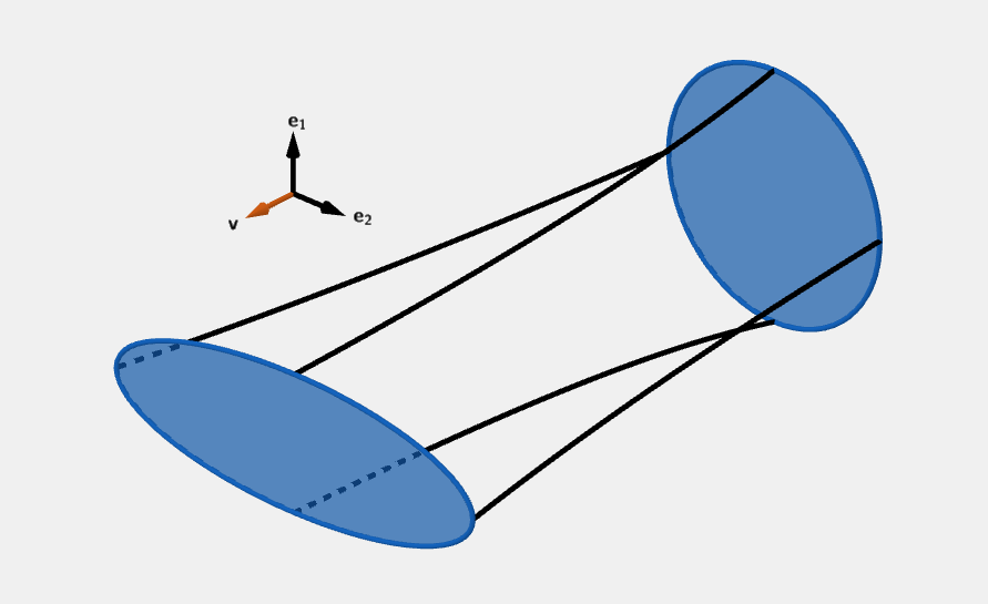
K ( s , v ) = 0 K(\boldsymbol{s}, \boldsymbol{v}) = 0 K ( s , v ) = 0 K ( s , v ) > 0 K(\boldsymbol{s}, \boldsymbol{v}) > 0 K ( s , v ) > 0 K ( s , v ) < 0 K(\boldsymbol{s}, \boldsymbol{v}) < 0 K ( s , v ) < 0 For Ricci curvature, we take a set of basis vectors { e 1 , e 2 , … , e n } \{\boldsymbol{e_1}, \boldsymbol{e_2}, \dots, \boldsymbol{e_n}\} { e 1 , e 2 , … , e n } v = e n \boldsymbol{v} = \boldsymbol{e_n} v = e n
R i c ( v , v ) = ∑ μ K ( e μ , v ) . Ric(\boldsymbol{v}, \boldsymbol{v}) = \sum_{\mu} K(\boldsymbol{e_{\mu}}, \boldsymbol{v}). R i c ( v , v ) = μ ∑ K ( e μ , v ) . In the scenario on the picture:
K ( e 1 , v ) > 0 , K ( e 2 , v ) < 0. \begin{align*} K(\boldsymbol{e_1}, \boldsymbol{v}) > 0, \\ K(\boldsymbol{e_2}, \boldsymbol{v}) < 0. \end{align*} K ( e 1 , v ) > 0 , K ( e 2 , v ) < 0. We don't have enough information, to determine the Ricci curvature, it could be positive, negative or even zero. If the Ricci curvature is zero, it implies the volume doesn't change, However from the Riemann tensor, we may still get that there is a curvature and a change in shape.
We can use the above formula and calculate the Ricci tensor components in orthonormal basis (dot product of same basis vectors is one and cross product of different basis vectors is zero):
R i c ( v , v ) = ∑ μ K ( e μ , v ) = ∑ μ [ R ( e μ , v ) v ] ⋅ e μ ( e μ ⋅ e μ ) ( v ⋅ v ) − ( e μ ⋅ v ) . = ∑ μ [ R ( e μ , v ) v ] ⋅ e μ ( 1 ) ( 1 ) − ( 0 ) = ∑ μ v ν v σ [ R ( e μ , e ν ) e σ ] ⋅ e μ = v ν v σ ∑ μ R λ σ μ ν e λ ⋅ e μ = v ν v σ ∑ μ R λ σ μ ν g λ μ = v ν v σ R μ σ μ ν = v ν v σ R σ ν , \begin{align*} Ric(\boldsymbol{v}, \boldsymbol{v}) &= \sum_{\mu} K(\boldsymbol{e_{\mu}}, \boldsymbol{v}) \\ &= \sum_{\mu} \frac{[R(\boldsymbol{e_{\mu}}, \boldsymbol{v}) \boldsymbol{v}] \cdot \boldsymbol{e_{\mu}}}{(\boldsymbol{e_{\mu}} \cdot \boldsymbol{e_{\mu}}) (\boldsymbol{v} \cdot \boldsymbol{v}) - (\boldsymbol{e_{\mu}} \cdot \boldsymbol{v})}. \\ &= \sum_{\mu} \frac{[R(\boldsymbol{e_{\mu}}, \boldsymbol{v}) \boldsymbol{v}] \cdot \boldsymbol{e_{\mu}}}{(1) (1) - (0)} \\ &= \sum_{\mu} v^{\nu} v^{\sigma} [R(\boldsymbol{e_{\mu}}, \boldsymbol{e_{\nu}}) \boldsymbol{e_{\sigma}}] \cdot \boldsymbol{e_{\mu}} \\ &= v^{\nu} v^{\sigma} \sum_{\mu} R^{\lambda}{}_{\sigma \mu \nu} \boldsymbol{e_{\lambda}} \cdot \boldsymbol{e_{\mu}} \\ &= v^{\nu} v^{\sigma} \sum_{\mu} R^{\lambda}{}_{\sigma \mu \nu} g_{\lambda \mu} \\ &= v^{\nu} v^{\sigma} R^{\mu}{}_{\sigma \mu \nu} \\ &= v^{\nu} v^{\sigma} R_{\sigma \nu}, \end{align*} R i c ( v , v ) = μ ∑ K ( e μ , v ) = μ ∑ ( e μ ⋅ e μ ) ( v ⋅ v ) − ( e μ ⋅ v ) [ R ( e μ , v ) v ] ⋅ e μ . = μ ∑ ( 1 ) ( 1 ) − ( 0 ) [ R ( e μ , v ) v ] ⋅ e μ = μ ∑ v ν v σ [ R ( e μ , e ν ) e σ ] ⋅ e μ = v ν v σ μ ∑ R λ σ μν e λ ⋅ e μ = v ν v σ μ ∑ R λ σ μν g λ μ = v ν v σ R μ σ μν = v ν v σ R σ ν , where
R σ ν = R μ σ μ ν R_{\sigma \nu} = R^{\mu}{}_{\sigma \mu \nu} R σ ν = R μ σ μν are the components of the Ricci tensor.
The step
∑ μ R λ σ μ ν g λ μ → R μ σ μ ν \sum_{\mu} R^{\lambda}{}_{\sigma \mu \nu} g_{\lambda \mu} \to R^{\mu}{}_{\sigma \mu \nu} μ ∑ R λ σ μν g λ μ → R μ σ μν might seem a bit weird at first, but remember that the metric tensor is the Kronecker delta. If we expand the sum, we get:
∑ μ R λ σ μ ν g λ μ = R λ σ 1 ν δ λ 1 + R λ σ 2 ν δ λ 2 + ⋯ = R 1 σ 1 ν + R 2 σ 2 ν + … . = R σ ν \sum_{\mu} R^{\lambda}{}_{\sigma \mu \nu} g_{\lambda \mu} = R^{\lambda}{}_{\sigma 1 \nu} \delta_{\lambda 1} + R^{\lambda}{}_{\sigma 2 \nu} \delta_{\lambda 2} + \dots = R^1{}_{\sigma 1 \nu} + R^2{}_{\sigma 2 \nu} + \dots. = R_{\sigma \nu} μ ∑ R λ σ μν g λ μ = R λ σ 1 ν δ λ 1 + R λ σ 2 ν δ λ 2 + ⋯ = R 1 σ 1 ν + R 2 σ 2 ν + … . = R σ ν Recall the components of the Riemann tensor:
R θ θ θ θ = 0 , R θ θ θ ϕ = 0 , R θ θ ϕ θ = 0 , R θ θ ϕ ϕ = 0 , R θ ϕ θ θ = 0 , R θ ϕ θ ϕ = sin 2 θ , R θ ϕ ϕ θ = − sin 2 θ , R θ ϕ ϕ ϕ = 0 , R ϕ θ θ θ = 0 , R ϕ θ θ ϕ = − 1 , R ϕ θ ϕ θ = 1 , R ϕ θ ϕ ϕ = 0 , R ϕ ϕ θ θ = 0 , R ϕ ϕ θ ϕ = 0 , R ϕ ϕ ϕ θ = 0 , R ϕ ϕ ϕ ϕ = 0. \begin{align*} R^{\theta}{}_{\theta \theta \theta} &= 0, & R^{\theta}{}_{\theta \theta \phi} &= 0, & R^{\theta}{}_{\theta \phi \theta} &= 0, & R^{\theta}{}_{\theta \phi \phi} &= 0, \\ R^{\theta}{}_{\phi \theta \theta} &= 0, & R^{\theta}{}_{\phi \theta \phi} &= \sin^2 \theta, & R^{\theta}{}_{\phi \phi \theta} &= - \sin^2 \theta, & R^{\theta}{}_{\phi \phi \phi} &= 0,\\ R^{\phi}{}_{\theta \theta \theta} &= 0, & R^{\phi}{}_{\theta \theta \phi} &= -1, & R^{\phi}{}_{\theta \phi \theta} &= 1, & R^{\phi}{}_{\theta \phi \phi} &= 0, \\ R^{\phi}{}_{\phi \theta \theta} &= 0, & R^{\phi}{}_{\phi \theta \phi} &= 0, & R^{\phi}{}_{\phi \phi \theta} &= 0, & R^{\phi}{}_{\phi \phi \phi} &= 0. \end{align*} R θ θθθ R θ ϕθθ R ϕ θθθ R ϕ ϕθθ = 0 , = 0 , = 0 , = 0 , R θ θθϕ R θ ϕθϕ R ϕ θθϕ R ϕ ϕθϕ = 0 , = sin 2 θ , = − 1 , = 0 , R θ θϕθ R θ ϕϕθ R ϕ θϕθ R ϕ ϕϕθ = 0 , = − sin 2 θ , = 1 , = 0 , R θ θϕϕ R θ ϕϕϕ R ϕ θϕϕ R ϕ ϕϕϕ = 0 , = 0 , = 0 , = 0. we can obtain the non zero components:
R θ θ = 1 , R ϕ ϕ = sin 2 θ . \begin{align*} R_{\theta \theta} &= 1, \\ R_{\phi \phi} &= \sin^2 \theta. \end{align*} R θθ R ϕϕ = 1 , = sin 2 θ . Sectional curvature works only in orthonormal basis. For any basis, we need to consider a different approach. We need to use the volume form which tells us the volume. For a parallelogram created by two vectors, the volume form is as follows:
ω ( u , v ) = ∣ u 1 v 1 u 2 v 2 ∣ = ϵ μ ν u μ v ν , \omega(\boldsymbol{u}, \boldsymbol{v}) = \begin{vmatrix} u^1 & v^1 \\ u^2 & v^2 \end{vmatrix} = \epsilon_{\mu \nu} u^{\mu} v^{\nu}, ω ( u , v ) = u 1 u 2 v 1 v 2 = ϵ μν u μ v ν , where
ϵ μ ν = { + 1 counting order ( ϵ 12 ) − 1 wrong order ( ϵ 21 ) 0 any index repeated \epsilon_{\mu \nu} = \begin{cases} +1 & \textrm{counting order (\(\epsilon_{12}\))} \\ -1 & \textrm{wrong order (\(\epsilon_{21}\))} \\ \ \ \ 0 & \textrm{any index repeated} \end{cases} ϵ μν = ⎩ ⎨ ⎧ + 1 − 1 0 counting order ( ϵ 12 ) wrong order ( ϵ 21 ) any index repeated is the Levi-Civita symbol.
A volume created by three vectors is equal to:
ω ( u , v , w ) = ∣ u 1 v 1 w 1 u 2 v 2 w 2 u 3 v 3 w 3 ∣ = ϵ μ ν σ u μ v ν w σ , \omega(\boldsymbol{u}, \boldsymbol{v}, \boldsymbol{w}) = \begin{vmatrix} u^1 & v^1 & w^1 \\ u^2 & v^2 & w^2 \\ u^3 & v^3 & w^3 \end{vmatrix} = \epsilon_{\mu \nu \sigma} u^{\mu} v^{\nu} w^{\sigma}, ω ( u , v , w ) = u 1 u 2 u 3 v 1 v 2 v 3 w 1 w 2 w 3 = ϵ μν σ u μ v ν w σ , where:
ϵ μ ν σ = { + 1 even permutation of μ ν σ − 1 odd permutation of μ ν σ 0 any index repeated \epsilon_{\mu \nu \sigma} = \begin{cases} +1 & \textrm{even permutation of \(\mu \nu \sigma\)} \\ -1 & \textrm{odd permutation of \(\mu \nu \sigma\)} \\ \ \ \ 0 & \textrm{any index repeated} \end{cases} ϵ μν σ = ⎩ ⎨ ⎧ + 1 − 1 0 even permutation of μν σ odd permutation of μν σ any index repeated Now this only works in orthonormal basis.
Just as we took the components of the vectors in orthonormal basis, we can take the volume form of an arbitrary basis obtained by a coordinate transformation from the orthonormal basis:
e ~ 1 = ∂ x 1 ∂ x ~ 1 e 1 + ∂ x 2 ∂ x ~ 1 e 2 , e ~ 2 = ∂ x 1 ∂ x ~ 2 e 1 + ∂ x 2 ∂ x ~ 2 e 2 , ω ( e ~ 1 , e ~ 2 ) = ∣ ∂ x 1 ∂ x ~ 1 ∂ x 1 ∂ x ~ 2 ∂ x 2 ∂ x ~ 1 ∂ x 2 ∂ x ~ 2 ∣ = det J , \begin{align*} \boldsymbol{\tilde{e}_1} &= \frac{\partial x^1}{\partial \tilde{x}^1} \boldsymbol{e_1} + \frac{\partial x^2}{\partial \tilde{x}^1} \boldsymbol{e_2}, \\ \boldsymbol{\tilde{e}_2} &= \frac{\partial x^1}{\partial \tilde{x}^2} \boldsymbol{e_1} + \frac{\partial x^2}{\partial \tilde{x}^2} \boldsymbol{e_2}, \\ \omega(\boldsymbol{\tilde{e}_1}, \boldsymbol{\tilde{e}_2}) &= \begin{vmatrix} \frac{\partial x^1}{\partial \tilde{x}^1} & \frac{\partial x^1}{\partial \tilde{x}^2} \\ \frac{\partial x^2}{\partial \tilde{x}^1} & \frac{\partial x^2}{\partial \tilde{x}^2} \end{vmatrix} = \det J, \end{align*} e ~ 1 e ~ 2 ω ( e ~ 1 , e ~ 2 ) = ∂ x ~ 1 ∂ x 1 e 1 + ∂ x ~ 1 ∂ x 2 e 2 , = ∂ x ~ 2 ∂ x 1 e 1 + ∂ x ~ 2 ∂ x 2 e 2 , = ∂ x ~ 1 ∂ x 1 ∂ x ~ 1 ∂ x 2 ∂ x ~ 2 ∂ x 1 ∂ x ~ 2 ∂ x 2 = det J , with the metric tensor transformed:
g ~ μ ν = ∂ x α ∂ x ~ μ ∂ x β ∂ x ~ ν g α β = J μ α J ν β g α β , \begin{align*} \tilde{g}_{\mu \nu} &= \frac{\partial x^{\alpha}}{\partial \tilde{x}^{\mu}} \frac{\partial x^{\beta}}{\partial \tilde{x}^{\nu}} g_{\alpha \beta} \\ &= J^{\alpha}_{\mu} J^{\beta}_{\nu} g_{\alpha \beta}, \end{align*} g ~ μν = ∂ x ~ μ ∂ x α ∂ x ~ ν ∂ x β g α β = J μ α J ν β g α β , and if we take the determinant of both sides, we obtain:
det g ~ = ( det J ) 2 ( det g ) = ( det J ) 2 , \det \tilde{g} = (\det J)^2 (\det g) = (\det J)^2, det g ~ = ( det J ) 2 ( det g ) = ( det J ) 2 , where the determinant of the old metric tensor is 1 since it's the Kronecker delta (orthonormal basis). This implies:
ω ( e 1 , e 2 ) = det g ~ . \omega(\boldsymbol{e_1}, \boldsymbol{e_2}) = \sqrt{\det \tilde{g}}. ω ( e 1 , e 2 ) = det g ~ . The volume form of the vectors in general basis is:
ω ( u , v ) = det g ∣ u 1 v 1 u 2 v 2 ∣ = det g ϵ μ ν u μ v ν , \omega(\boldsymbol{u}, \boldsymbol{v}) = \sqrt{\det g} \begin{vmatrix} u^1 & v^1 \\ u^2 & v^2 \end{vmatrix} = \sqrt{\det g} \epsilon_{\mu \nu} u^{\mu} v^{\nu}, ω ( u , v ) = det g u 1 u 2 v 1 v 2 = det g ϵ μν u μ v ν , where I have relabeled g ~ \tilde{g} g ~ g g g
ω ( u , v , w ) = det g ∣ u 1 v 1 w 1 u 2 v 2 w 2 u 3 v 3 w 3 ∣ = det g ϵ μ ν σ u μ v ν w σ , \omega(\boldsymbol{u}, \boldsymbol{v}, \boldsymbol{w}) = \sqrt{\det g} \begin{vmatrix} u^1 & v^1 & w^1 \\ u^2 & v^2 & w^2 \\ u^3 & v^3 & w^3 \end{vmatrix} = \sqrt{\det g}\ \epsilon_{\mu \nu \sigma} u^{\mu} v^{\nu} w^{\sigma}, ω ( u , v , w ) = det g u 1 u 2 u 3 v 1 v 2 v 3 w 1 w 2 w 3 = det g ϵ μν σ u μ v ν w σ , or in general:
ω ( v 1 , v 2 , … ) = det g ϵ α β … v 1 α v 2 β ⋯ = det g ϵ μ 1 μ 2 … ( ∏ i v i μ i ) , \omega(\boldsymbol{v_1}, \boldsymbol{v_2}, \dots) = \sqrt{\det g}\ \epsilon_{\alpha \beta \dots} v_1^{\alpha} v_2^{\beta} \dots = \sqrt{\det g}\ \epsilon_{\mu_1 \mu_2 \dots} \left(\prod_{i} v_i^{\mu_i}\right), ω ( v 1 , v 2 , … ) = det g ϵ α β … v 1 α v 2 β ⋯ = det g ϵ μ 1 μ 2 … ( i ∏ v i μ i ) , where there is a sum for each μ i \mu_i μ i
I will prove that the first covariant derivative is zero. We take a geodesic path and parallel transport the vectors along the path. And since the Levi-Civita connection preserves, volume, the covariant derivative of the volume form must be zero:
0 = ∇ u ω ( v 1 , v 1 , … ) = ( ∏ i v i μ i ) ∇ u det g ϵ μ 1 μ 2 … = 0 , 0 = \nabla_{\boldsymbol{u}} \omega(\boldsymbol{v_1}, \boldsymbol{v_1}, \dots) = \left(\prod_{i} v_i^{\mu_i}\right) \nabla_{\boldsymbol{u}} \sqrt{\det g}\ \epsilon_{\mu_1 \mu_2 \dots} = 0, 0 = ∇ u ω ( v 1 , v 1 , … ) = ( i ∏ v i μ i ) ∇ u det g ϵ μ 1 μ 2 … = 0 , where the product can go outside the covariant derivative, since by the definition of parallel transport, its covariant derivative is zero. Note that this does not mean that the volume does not change. Just that the way we measure volume does not change. Now let's take the second covariant derivative of a volume spanned by separation vectors between geodesics:
V = det g ϵ μ 1 μ 2 … ( ∏ i s i μ i ) , ∇ v ∇ v V = ∇ v ∇ v [ det g ϵ μ 1 μ 2 … ( ∏ i s i μ i ) ] = det g ϵ μ 1 μ 2 … ∇ v ∇ v ( ∏ i s i μ i ) = det g ϵ μ 1 μ 2 … ∇ v ( s ˙ j μ j ∏ i ≠ j s i μ i ) = det g ϵ μ 1 μ 2 … ( s ¨ j μ j ∏ i ≠ j s i μ i + s ˙ i μ j s ˙ k μ k ∏ i ≠ j , k s i μ i ) , \begin{align*} V &= \sqrt{\det g}\ \epsilon_{\mu_1 \mu_2 \dots} \left(\prod_{i} s_i^{\mu_i}\right), \\ \nabla_{\boldsymbol{v}} \nabla_{\boldsymbol{v}} V = \nabla_{\boldsymbol{v}} \nabla_{\boldsymbol{v}} \left[\sqrt{\det g}\ \epsilon_{\mu_1 \mu_2 \dots} \left(\prod_{i} s_i^{\mu_i}\right)\right] &= \sqrt{\det g}\ \epsilon_{\mu_1 \mu_2 \dots} \nabla_{\boldsymbol{v}} \nabla_{\boldsymbol{v}} \left(\prod_{i} s_i^{\mu_i}\right) \\ &= \sqrt{\det g}\ \epsilon_{\mu_1 \mu_2 \dots} \nabla_{\boldsymbol{v}} \left(\dot{s}_j^{\mu_j} \prod_{i \neq j} s_i^{\mu_i}\right) \\ &= \sqrt{\det g}\ \epsilon_{\mu_1 \mu_2 \dots} \left(\ddot{s}_j^{\mu_j} \prod_{i \neq j} s_i^{\mu_i} + \dot{s}_i^{\mu_j} \dot{s}_k^{\mu_k} \prod_{i \neq j, k} s_i^{\mu_i}\right), \end{align*} V ∇ v ∇ v V = ∇ v ∇ v [ det g ϵ μ 1 μ 2 … ( i ∏ s i μ i ) ] = det g ϵ μ 1 μ 2 … ( i ∏ s i μ i ) , = det g ϵ μ 1 μ 2 … ∇ v ∇ v ( i ∏ s i μ i ) = det g ϵ μ 1 μ 2 … ∇ v s ˙ j μ j i = j ∏ s i μ i = det g ϵ μ 1 μ 2 … s ¨ j μ j i = j ∏ s i μ i + s ˙ i μ j s ˙ k μ k i = j , k ∏ s i μ i , since s i \boldsymbol{s_i} s i
∇ v ∇ v s = − R ( s , v ) v = − R σ λ α β s α v β v λ e σ , ( ∇ v ∇ v s ) σ = − R σ λ α β s α v β v λ , s ¨ j μ j = − R μ j λ α β s j α v β v λ \begin{align*} \nabla_{\boldsymbol{v}} \nabla_{\boldsymbol{v}} \boldsymbol{s} &= -R(\boldsymbol{s}, \boldsymbol{v}) \boldsymbol{v} \\ &= - R^{\sigma}{}_{\lambda \alpha \beta} s^{\alpha} v^{\beta} v^{\lambda} \boldsymbol{e_{\sigma}}, \\ (\nabla_{\boldsymbol{v}} \nabla_{\boldsymbol{v}} \boldsymbol{s})^{\sigma} &= - R^{\sigma}{}_{\lambda \alpha \beta} s^{\alpha} v^{\beta} v^{\lambda}, \\ \ddot{s}_j^{\mu_j} &= - R^{\mu_j}{}_{\lambda \alpha \beta} s_j^{\alpha} v^{\beta} v^{\lambda} \end{align*} ∇ v ∇ v s ( ∇ v ∇ v s ) σ s ¨ j μ j = − R ( s , v ) v = − R σ λ α β s α v β v λ e σ , = − R σ λ α β s α v β v λ , = − R μ j λ α β s j α v β v λ continuing:
∇ v ∇ v V = det g ϵ μ 1 μ 2 … ( − R μ j λ α β s j α v β v λ ∏ i ≠ j s i μ i + s ˙ i μ j s ˙ k μ k ∏ i ≠ j , k s i μ i ) . \nabla_{\boldsymbol{v}} \nabla_{\boldsymbol{v}} V = \sqrt{\det g}\ \epsilon_{\mu_1 \mu_2 \dots} \left(- R^{\mu_j}{}_{\lambda \alpha \beta} s_j^{\alpha} v^{\beta} v^{\lambda} \prod_{i \neq j} s_i^{\mu_i} + \dot{s}_i^{\mu_j} \dot{s}_k^{\mu_k} \prod_{i \neq j, k} s_i^{\mu_i}\right). ∇ v ∇ v V = det g ϵ μ 1 μ 2 … − R μ j λ α β s j α v β v λ i = j ∏ s i μ i + s ˙ i μ j s ˙ k μ k i = j , k ∏ s i μ i . Remember, there are summations across the μ i \mu_i μ i μ j \mu_j μ j α = μ j \alpha = \mu_j α = μ j
∇ v ∇ v V = det g ϵ μ 1 μ 2 … ( − R μ j λ μ j β s j μ j v β v λ ∏ i ≠ j s i μ i + s ˙ i μ j s ˙ k μ k ∏ i ≠ j , k s i μ i ) = − R μ j λ μ j β v β v λ det g ϵ μ 1 μ 2 … ∏ i s i μ i + det g ϵ μ 1 μ 2 … s ˙ i μ j s ˙ k μ k ∏ i ≠ j , k s i μ i = − R λ β v β v λ V + det g ϵ μ 1 μ 2 … s ˙ i μ j s ˙ k μ k ∏ i ≠ j , k s i μ i , \begin{align*} \nabla_{\boldsymbol{v}} \nabla_{\boldsymbol{v}} V &= \sqrt{\det g}\ \epsilon_{\mu_1 \mu_2 \dots} \left(- R^{\mu_j}{}_{\lambda \mu_j \beta} s_j^{\mu_j} v^{\beta} v^{\lambda} \prod_{i \neq j} s_i^{\mu_i} + \dot{s}_i^{\mu_j} \dot{s}_k^{\mu_k} \prod_{i \neq j, k} s_i^{\mu_i}\right) \\ &= -R^{\mu_j}{}_{\lambda \mu_j \beta} v^{\beta} v^{\lambda} \sqrt{\det g}\ \epsilon_{\mu_1 \mu_2 \dots} \prod_i s_i^{\mu_i} + \sqrt{\det g}\ \epsilon_{\mu_1 \mu_2 \dots} \dot{s}_i^{\mu_j} \dot{s}_k^{\mu_k} \prod_{i \neq j, k} s_i^{\mu_i} \\ &= -R_{\lambda \beta} v^{\beta} v^{\lambda} V + \sqrt{\det g}\ \epsilon_{\mu_1 \mu_2 \dots} \dot{s}_i^{\mu_j} \dot{s}_k^{\mu_k} \prod_{i \neq j, k} s_i^{\mu_i}, \end{align*} ∇ v ∇ v V = det g ϵ μ 1 μ 2 … − R μ j λ μ j β s j μ j v β v λ i = j ∏ s i μ i + s ˙ i μ j s ˙ k μ k i = j , k ∏ s i μ i = − R μ j λ μ j β v β v λ det g ϵ μ 1 μ 2 … i ∏ s i μ i + det g ϵ μ 1 μ 2 … s ˙ i μ j s ˙ k μ k i = j , k ∏ s i μ i = − R λ β v β v λ V + det g ϵ μ 1 μ 2 … s ˙ i μ j s ˙ k μ k i = j , k ∏ s i μ i , where R λ β R_{\lambda \beta} R λ β
Since the Ricci tensor components are all positive on the surface of a sphere, this means that the first component is negative. This means that the volumes shrink.
The Ricci scalar keeps track of how the size of a ball deviates from the size in flat space:
R = R μ μ = g μ ν R μ ν . R = R^{\mu}{}_{\mu} = g^{\mu \nu} R_{\mu \nu}. R = R μ μ = g μν R μν . On the surface of the sphere, this equals to:
R = g θ θ R θ θ + g ϕ ϕ R ϕ ϕ = 1 r 2 + 1 r 2 sin 2 θ sin 2 θ = 2 r 2 . R = g^{\theta \theta} R_{\theta \theta} + g^{\phi \phi} R_{\phi \phi} = \frac{1}{r^2} + \frac{1}{r^2 \sin^2 \theta} \sin^2 \theta = \frac{2}{r^2}. R = g θθ R θθ + g ϕϕ R ϕϕ = r 2 1 + r 2 sin 2 θ 1 sin 2 θ = r 2 2 . I will replace the radius of the sphere r r r R \mathcal{R} R
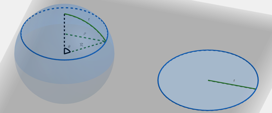
R = 2 R 2 . R = \frac{2}{\mathcal{R}^2}. R = R 2 2 . Observe the difference between circle on the surface of a sphere vs a circle in flat space:
We can see that the circle on the surface of a sphere has bigger area. Also:
r = R θ , ρ = R sin θ . \begin{align*} r &= \mathcal{R} \theta, \\ \rho &= \mathcal{R} \sin \theta. \end{align*} r ρ = R θ , = R sin θ . The area of the flat circle is:
A f = π r 2 , A_f = \pi r^2, A f = π r 2 , while the area of the circle on the surface of the sphere is:
A s = ∫ d A = ∫ 2 π ρ d r = ∫ 2 π R sin θ R d θ = 2 π R 2 ∫ 0 θ sin θ d θ = − 2 π R 2 [ cos θ ] 0 θ = 2 π R 2 ( 1 − cos θ ) = 2 π R 2 ( 1 − cos r R ) . \begin{align*} A_s &= \int dA \\ &= \int 2 \pi \rho\ dr \\ &= \int 2 \pi \mathcal{R} \sin \theta \mathcal{R} d \theta \\ &= 2 \pi \mathcal{R}^2 \int_0^{\theta}\sin \theta d \theta \\ &= -2 \pi \mathcal{R}^2 \left[\cos \theta\right]_0^{\theta} \\ &= 2 \pi \mathcal{R}^2 (1 - \cos \theta) \\ &= 2 \pi \mathcal{R}^2 \left(1 - \cos \frac{r}{\mathcal{R}}\right). \end{align*} A s = ∫ d A = ∫ 2 π ρ d r = ∫ 2 π R sin θ R d θ = 2 π R 2 ∫ 0 θ sin θ d θ = − 2 π R 2 [ cos θ ] 0 θ = 2 π R 2 ( 1 − cos θ ) = 2 π R 2 ( 1 − cos R r ) . The ratio of the curved and flat area is:
A s A f = 2 π R 2 ( 1 − cos r R ) π r 2 = 2 R 2 ( 1 − cos r R ) r 2 . \begin{align*} \frac{A_s}{A_f} &= \frac{2 \pi \mathcal{R}^2 \left(1 - \cos \frac{r}{\mathcal{R}}\right)}{\pi r^2} \\ &= \frac{2 \mathcal{R}^2 \left(1 - \cos \frac{r}{\mathcal{R}}\right)}{r^2}. \end{align*} A f A s = π r 2 2 π R 2 ( 1 − cos R r ) = r 2 2 R 2 ( 1 − cos R r ) . I will take the taylor series of the cosine:
A s A f = 2 R 2 r 2 ( 1 − ( 1 − 1 2 ! ( r R ) 2 + 1 4 ! ( r R ) 4 − 1 6 ! ( r R ) 6 + ⋯ ) ) = 2 R 2 r 2 ( 1 2 ! ( r R ) 2 − 1 4 ! ( r R ) 4 + 1 6 ! ( r R ) 6 − ⋯ ) = 1 − r 2 24 2 R 2 + 2 [ 1 6 ! ( r R ) 4 − ⋯ ] = 1 − r 2 24 2 R 2 + 2 [ 1 6 ! ( r R ) 4 − ⋯ ] = 1 − r 2 24 R + [ O ( r ) 4 + ⋯ ] , \begin{align*} \frac{A_s}{A_f} &= \frac{2 \mathcal{R}^2}{r^2} \left(1 - \left(1 - \frac{1}{2!} \left(\frac{r}{\mathcal{R}}\right)^2 + \frac{1}{4!} \left(\frac{r}{\mathcal{R}}\right)^4 - \frac{1}{6!} \left(\frac{r}{\mathcal{R}}\right)^6 + \cdots \right)\right) \\ &= \frac{2 \mathcal{R}^2}{r^2} \left(\frac{1}{2!} \left(\frac{r}{\mathcal{R}}\right)^2 - \frac{1}{4!} \left(\frac{r}{\mathcal{R}}\right)^4 + \frac{1}{6!} \left(\frac{r}{\mathcal{R}}\right)^6 - \cdots\right) \\ &= 1 - \frac{r^2}{24} \frac{2}{\mathcal{R}^2} + 2 \left[\frac{1}{6!} \left(\frac{r}{\mathcal{R}}\right)^4 - \cdots\right] \\ &= 1 - \frac{r^2}{24} \frac{2}{\mathcal{R}^2} + 2 \left[\frac{1}{6!} \left(\frac{r}{\mathcal{R}}\right)^4 - \cdots\right] \\ &= 1 - \frac{r^2}{24} R + \left[O(r)^4 + \cdots\right], \end{align*} A f A s = r 2 2 R 2 ( 1 − ( 1 − 2 ! 1 ( R r ) 2 + 4 ! 1 ( R r ) 4 − 6 ! 1 ( R r ) 6 + ⋯ ) ) = r 2 2 R 2 ( 2 ! 1 ( R r ) 2 − 4 ! 1 ( R r ) 4 + 6 ! 1 ( R r ) 6 − ⋯ ) = 1 − 24 r 2 R 2 2 + 2 [ 6 ! 1 ( R r ) 4 − ⋯ ] = 1 − 24 r 2 R 2 2 + 2 [ 6 ! 1 ( R r ) 4 − ⋯ ] = 1 − 24 r 2 R + [ O ( r ) 4 + ⋯ ] , this ratio is a little less than one. Meaning for the same radius (r r r ρ \rho ρ
Generally, if a Ricci scalar is positive, it means that for the same radius, curved space has less area. And for the same circumference, curved space has more area.
If a Ricci scalar is negative, it means that for the same radius, curved space has more area. And for the same circumference, curved space has less area.
Recall the symmetries and identities of the Riemann tensor:
R σ ρ μ λ = − R σ ρ λ μ , R σ γ α β + R σ β γ α + R σ α β γ = 0 , R β α μ λ = − R α β μ λ , R σ γ α β = R α β σ γ . \begin{align*} R_{\sigma \rho \mu \lambda} &= -R_{\sigma \rho \lambda \mu}, \\ R_{\sigma \gamma \alpha \beta} + R_{\sigma \beta \gamma \alpha} + R_{\sigma \alpha \beta \gamma} &= 0, \tag{Torsion-free} \\ R_{\beta \alpha \mu \lambda} &= -R_{\alpha \beta \mu \lambda}, \tag{Metric compatibility} \\ R_{\sigma \gamma \alpha \beta} &= R_{\alpha \beta \sigma \gamma}. \tag{Torsion-free \& metric compatibility} \\ \end{align*} R σ ρ μ λ R σγ α β + R σ β γ α + R σ α β γ R β αμ λ R σγ α β = − R σ ρ λ μ , = 0 , = − R α β μ λ , = R α β σγ . ( Torsion-free ) ( Metric compatibility ) ( Torsion-free & metric compatibility ) The Ricci tensor is a contraction of the Riemann tensor:
R μ ν = R σ μ σ ν = g σ λ R λ μ σ ν . R_{\mu \nu} = R^{\sigma}{}_{\mu \sigma \nu} = g^{\sigma \lambda} R_{\lambda \mu \sigma \nu}. R μν = R σ μ σ ν = g σλ R λ μ σ ν . Consider the contraction in the contravariant index and the first covariant index:
R σ σ μ ν = g σ λ R λ σ μ ν = − g σ λ R σ λ μ ν = 0. R^{\sigma}{}_{\sigma \mu \nu} = g^{\sigma \lambda} R_{\lambda \sigma \mu \nu} = -g^{\sigma \lambda} R_{\sigma \lambda \mu \nu} = 0. R σ σ μν = g σλ R λσ μν = − g σλ R σλ μν = 0. We already know that the contraction in the contravariant index and the second covariant index is the Ricci tensor components:
R σ μ σ ν = R μ ν . R^{\sigma}{}_{\mu \sigma \nu} = R_{\mu \nu}. R σ μ σ ν = R μν . Considering the last possibility - the contraction in the contravariant index and the third covariant index:
R σ μ ν σ = g σ λ R λ μ ν σ = − g σ λ R λ μ σ ν = − R μ ν , R^{\sigma}{}_{\mu \nu \sigma} = g^{\sigma \lambda} R_{\lambda \mu \nu \sigma} = -g^{\sigma \lambda} R_{\lambda \mu \sigma \nu} = -R_{\mu \nu}, R σ μν σ = g σλ R λ μν σ = − g σλ R λ μ σ ν = − R μν , so the Ricci tensor is the only meaningful contraction.
The Ricci tensor is symmetric:
R μ ν = g σ λ R λ μ σ ν = g σ λ R σ ν λ μ = R ν μ . \begin{align*} R_{\mu \nu} &= g^{\sigma \lambda} R_{\lambda \mu \sigma \nu} \\ &= g^{\sigma \lambda} R_{\sigma \nu \lambda \mu} \\ &= R_{\nu \mu}. \end{align*} R μν = g σλ R λ μ σ ν = g σλ R σ ν λ μ = R νμ . Recall the second Bianchi identity:
R σ λ α β ; γ + R σ λ γ α ; β + R σ λ β γ ; α = 0 , R^{\sigma}{}_{\lambda \alpha \beta; \gamma} + R^{\sigma}{}_{\lambda \gamma \alpha; \beta} + R^{\sigma}{}_{\lambda \beta \gamma; \alpha} = 0, R σ λ α β ; γ + R σ λγ α ; β + R σ λ β γ ; α = 0 , I will lower the index and do the following contraction:
R σ λ α β ; γ + R σ λ γ α ; β + R σ λ β γ ; α = 0 , g λ β g σ α ( R σ λ α β ; γ + R σ λ γ α ; β + R σ λ β γ ; α ) = 0 , g λ β ( R α λ α β ; γ + R α λ γ α ; β + g σ α R σ λ β γ ; α ) = 0 , g λ β ( R λ β ; γ − R α λ α γ ; β − g σ α R λ σ β γ ; α ) = 0 , R β β ; γ − g λ β R λ γ ; β − g σ α R β σ β γ ; α = 0 , R ; γ − R β γ ; β − g σ α R σ γ ; α = 0 , R ; γ − R β γ ; β − R α γ ; α = 0 , R ; γ − R β γ ; β − R β γ ; β = 0 , R ; γ − 2 R β γ ; β = 0 , 1 2 δ γ β R ; β − R β γ ; β = 0 , 1 2 g γ ρ δ γ β R ; β − g γ ρ R β γ ; β = 0 , 1 2 g β ρ R ; β − R β ρ ; β = 0 , \begin{align*} R_{\sigma \lambda \alpha \beta; \gamma} + R_{\sigma \lambda \gamma \alpha; \beta} + R_{\sigma \lambda \beta \gamma; \alpha} &= 0, \\ g^{\lambda \beta} g^{\sigma \alpha} (R_{\sigma \lambda \alpha \beta; \gamma} + R_{\sigma \lambda \gamma \alpha; \beta} + R_{\sigma \lambda \beta \gamma; \alpha}) &= 0, \\ g^{\lambda \beta} (R^{\alpha}{}_{\lambda \alpha \beta; \gamma} + R^{\alpha}{}_{\lambda \gamma \alpha; \beta} + g^{\sigma \alpha} R_{\sigma \lambda \beta \gamma; \alpha}) &= 0, \\ g^{\lambda \beta} (R_{\lambda \beta; \gamma} - R^{\alpha}{}_{\lambda \alpha \gamma; \beta} - g^{\sigma \alpha} R_{\lambda \sigma \beta \gamma; \alpha}) &= 0, \\ R^{\beta}{}_{\beta; \gamma} - g^{\lambda \beta} R_{\lambda \gamma; \beta} - g^{\sigma \alpha} R^{\beta}{}_{\sigma \beta \gamma; \alpha} &= 0, \\ R_{; \gamma} - R^{\beta}{}_{\gamma; \beta} - g^{\sigma \alpha} R_{\sigma \gamma; \alpha} &= 0, \\ R_{; \gamma} - R^{\beta}{}_{\gamma; \beta} - R^{\alpha}{}_{\gamma; \alpha} &= 0, \\ R_{; \gamma} - R^{\beta}{}_{\gamma; \beta} - R^{\beta}{}_{\gamma; \beta} &= 0, \\ R_{; \gamma} - 2 R^{\beta}{}_{\gamma; \beta} &= 0, \\ \frac{1}{2} \delta^{\beta}_{\gamma} R_{; \beta} - R^{\beta}{}_{\gamma; \beta} &= 0, \\ \frac{1}{2} g^{\gamma \rho} \delta^{\beta}_{\gamma} R_{; \beta} - g^{\gamma \rho} R^{\beta}{}_{\gamma; \beta} &= 0, \\ \frac{1}{2} g^{\beta \rho} R_{; \beta} - R^{\beta \rho}{}_{; \beta} &= 0, \end{align*} R σλ α β ; γ + R σλγ α ; β + R σλ β γ ; α g λ β g σ α ( R σλ α β ; γ + R σλγ α ; β + R σλ β γ ; α ) g λ β ( R α λ α β ; γ + R α λγ α ; β + g σ α R σλ β γ ; α ) g λ β ( R λ β ; γ − R α λ α γ ; β − g σ α R λσ β γ ; α ) R β β ; γ − g λ β R λγ ; β − g σ α R β σ β γ ; α R ; γ − R β γ ; β − g σ α R σγ ; α R ; γ − R β γ ; β − R α γ ; α R ; γ − R β γ ; β − R β γ ; β R ; γ − 2 R β γ ; β 2 1 δ γ β R ; β − R β γ ; β 2 1 g γ ρ δ γ β R ; β − g γ ρ R β γ ; β 2 1 g βρ R ; β − R βρ ; β = 0 , = 0 , = 0 , = 0 , = 0 , = 0 , = 0 , = 0 , = 0 , = 0 , = 0 , = 0 , and this is called the contracted Bianchi identity:
R α β ; β − 1 2 g α β R ; β = 0. R^{\alpha \beta}{}_{; \beta} - \frac{1}{2} g^{\alpha \beta} R_{; \beta} = 0. R α β ; β − 2 1 g α β R ; β = 0. This can be rewritten:
R α β ; β − 1 2 g α β R ; β = 0 , ( R α β − 1 2 g α β R ) ; β = 0 , G α β ; β = 0. \begin{align*} R^{\alpha \beta}{}_{; \beta} - \frac{1}{2} g^{\alpha \beta} R_{; \beta} &= 0, \\ \left(R^{\alpha \beta} - \frac{1}{2} g^{\alpha \beta} R\right)_{; \beta} &= 0, \\ G^{\alpha \beta}{}_{; \beta} &= 0. \end{align*} R α β ; β − 2 1 g α β R ; β ( R α β − 2 1 g α β R ) ; β G α β ; β = 0 , = 0 , = 0. where
G α β = R α β − 1 2 g α β R G^{\alpha \beta} = R^{\alpha \beta} - \frac{1}{2} g^{\alpha \beta} R G α β = R α β − 2 1 g α β R is the Einstein tensor.
The conservation of energy-momentum is as follows:
T α β ; β = 0 , T^{\alpha \beta}{}_{; \beta} = 0, T α β ; β = 0 , where T α β T^{\alpha \beta} T α β
This implies:
G α β ; β = T α β ; β = 0. G^{\alpha \beta}{}_{; \beta} = T^{\alpha \beta}{}_{;\beta} = 0. G α β ; β = T α β ; β = 0. We can say that the curvature is proportional to the energy and momentum:
G α β = 8 π G c 4 T α β , R α β − 1 2 g α β R = 8 π G c 4 T α β , \begin{align*} G^{\alpha \beta} &= \frac{8 \pi G}{c^4} T^{\alpha \beta}, \\ R^{\alpha \beta} - \frac{1}{2} g^{\alpha \beta} R &= \frac{8 \pi G}{c^4} T^{\alpha \beta}, \end{align*} G α β R α β − 2 1 g α β R = c 4 8 π G T α β , = c 4 8 π G T α β , where all three tensors are symmetric. In four dimensional spacetime, this results in ten independent equations.
Since the covariant derivative is zero, we can add the metric tensor multiplied by a constant:
R α β − 1 2 g α β R + Λ g α β = 8 π G c 4 T α β , R^{\alpha \beta} - \frac{1}{2} g^{\alpha \beta} R + \Lambda g^{\alpha \beta} = \frac{8 \pi G}{c^4} T^{\alpha \beta}, R α β − 2 1 g α β R + Λ g α β = c 4 8 π G T α β , or in the covariant form:
R α β − 1 2 g α β R + Λ g α β = 8 π G c 4 T α β , R_{\alpha \beta} - \frac{1}{2} g_{\alpha \beta} R + \Lambda g_{\alpha \beta} = \frac{8 \pi G}{c^4} T_{\alpha \beta}, R α β − 2 1 g α β R + Λ g α β = c 4 8 π G T α β , where Λ \Lambda Λ