BackRiemann Tensor
To naively define flat space, we could say that space is flat when all Γσμν=0. However, when dealing with polar coordinates in flat space, there are nonzero connection coefficients.
A second attempt would be to define space as flat, when we can make Γσμν=0 by a change of coordinates. This attempt however fails when we consider the surface of a sphere with radius equal to one. If we set θ=2π, the metric is the Kronecker delta and the Christoffel components are zero:
gμνΓθϕϕΓϕθϕ=Γϕϕθ=[r200r2sin2θ]=[1001]=δμν,=−sinθcosθ=0,=cotθ=0. And we can rotate the coordinate system such that any point lies on the equator on the sphere.
It turns out, that on any manifold, we can always find a special coordinate system called the Riemann normal coordinates at point p, where the following is true at that point:
gμνΓσμν=δμν,=0. So to detect curvature, we need a new tool called the Riemann tensor.
Remember that a vector may rotate when performing parallel transport:
this is called holonomy and I will use it to define the Riemann tensor.
Instead of doing parallel transform, we could do a related computation - the commutator of the covariant derivative. So we are measuring the change from the change from parallel transport and comparing it with the change from the change from parallel transport if we take the opposite route:
[∇u,∇v]w=∇u∇vw−∇v∇uw, The covariant derivatives are computed the same way, the second has swapped u and v:
∇u∇vw∇v∇uw[∇u,∇v]w=uμ(∂xμ∂(∇vw)σ+(∇vw)νΓσμν)eσ=uμ(∂xμ∂(vλ(∂xλ∂wσ+wρΓσλρ))+vλ(∂xλ∂wν+wρΓνλρ)Γσμν)eσ=uμ(∂xμ∂vλ(∂xλ∂wσ+wρΓσλρ)+vλ∂xμ∂(∂xλ∂wσ+wρΓσλρ)+vλ(∂xλ∂wν+wρΓνλρ)Γσμν)eσ=uμ(∂xμ∂vλ∂xλ∂wσ+∂xμ∂vλwρΓσλρ+vλ∂xμ∂xλ∂2wσ+vλ∂xμ∂(wρΓσλρ)+vλ∂xλ∂wνΓσμν+vλwρΓνλρΓσμν)eσ=uμ(∂xμ∂vλ∂xλ∂wσ+∂xμ∂vλwρΓσλρ+vλ∂xμ∂xλ∂2wσ+vλ∂xμ∂wρΓσλρ+vλwρ∂xμ∂Γσλρ+vλ∂xλ∂wνΓσμν+vλwρΓνλρΓσμν)eσ=(uμ∂xμ∂vλ∂xλ∂wσ+uμ∂xμ∂vλwρΓσλρ+uμvλ∂xμ∂xλ∂2wσ+uμvλ∂xμ∂wρΓσλρ+uμvλwρ∂xμ∂Γσλρ+uμvλ∂xλ∂wνΓσμν+uμvλwρΓνλρΓσμν)eσ=(vμ∂xμ∂uλ∂xλ∂wσ+vμ∂xμ∂uλwρΓσλρ+vμuλ∂xμ∂xλ∂2wσ+vμuλ∂xμ∂wρΓσλρ+vμuλwρ∂xμ∂Γσλρ+vμuλ∂xλ∂wνΓσμν+vμuλwρΓνλρΓσμν)eσ=(uμ∂xμ∂vλ∂xλ∂wσ+uμ∂xμ∂vλwρΓσλρ+uμvλ∂xμ∂xλ∂2wσ+uμvλ∂xμ∂wρΓσλρ+uμvλwρ∂xμ∂Γσλρ+uμvλ∂xλ∂wνΓσμν+uμvλwρΓνλρΓσμν−vμ∂xμ∂uλ∂xλ∂wσ−vμ∂xμ∂uλwρΓσλρ−vμuλ∂xμ∂xλ∂2wσ−vμuλ∂xμ∂wρΓσλρ−vμuλwρ∂xμ∂Γσλρ−vμuλ∂xλ∂wνΓσμν−vμuλwρΓνλρΓσμν)eσ=(uμ∂xμ∂vλ∂xλ∂wσ+uμ∂xμ∂vλwρΓσλρ+uμvλ∂xμ∂xλ∂2wσ+uμvλ∂xμ∂wρΓσλρ+uμvλwρ∂xμ∂Γσλρ+uμvλ∂xλ∂wνΓσμν+uμvλwρΓνλρΓσμν−vμ∂xμ∂uλ∂xλ∂wσ−vμ∂xμ∂uλwρΓσλρ−vλuμ∂xλ∂xμ∂2wσ−vλuμ∂xλ∂wνΓσμν−vμuλwρ∂xμ∂Γσλρ−vλuμ∂xμ∂wρΓσλρ−vμuλwρΓνλρΓσμν)eσ=(uμ∂xμ∂vλ∂xλ∂wσ+uμwρ∂xμ∂vλΓσλρ+uμwρvλ∂xμ∂Γσλρ+uμvλwρΓνλρΓσμν−vμ∂xμ∂uλ∂xλ∂wσ−vμwρ∂xμ∂uλΓσλρ−vμwρuλ∂xμ∂Γσλρ−uλvμwρΓνλρΓσμν)eσ=(uμ∂xμ∂vλ∂xλ∂wσ+uμwρ∂xμ∂vλΓσλρ+uμvλwρ∂xμ∂Γσλρ+uμvλwρΓνλρΓσμν−vμ∂xμ∂uλ∂xλ∂wσ−vμwρ∂xμ∂uλΓσλρ−uμvλwρ∂xλ∂Γσμρ−uμvλwρΓνμρΓσλν)eσ=uμ∂xμ∂vλ(∂xλ∂wσ+wρΓσλρ)eσ−vμ∂xμ∂uλ(∂xλ∂wσ+wρΓσλρ)eσ+uμvλwρ(∂xμ∂Γσλρ−∂xλ∂Γσμρ+ΓνλρΓσμν−ΓνμρΓσλν)eσ=(∂xμ∂vλuμ−vμ∂xμ∂uλ)(∂xλ∂wσ+wρΓσλρ)eσ+uμvλwρ(∂xμ∂Γσλρ−∂xλ∂Γσμρ+ΓνλρΓσμν−ΓνμρΓσλν)eσ=(∂xμ∂vλuμ−vμ∂xμ∂uλ)∇eλw+uμvλwρ(∂xμ∂Γσλρ−∂xλ∂Γσμρ+ΓνλρΓσμν−ΓνμρΓσλν)eσ=(uμ∂μvλ−vμ∂μuλ)∇eλw+uμvλwρ(∂xμ∂Γσλρ−∂xλ∂Γσμρ+ΓνλρΓσμν−ΓνμρΓσλν)eσ=∇uμ∂μvλ∂λ−vμ∂μuλ∂λw+uμvλwρ(∂xμ∂Γσλρ−∂xλ∂Γσμρ+ΓνλρΓσμν−ΓνμρΓσλν)eσ. The term in the covariant derivative is the Lie bracket (remember, the order of partial differentiation does not matter):
uμ∂μvλ∂λ−vμ∂μuλ∂λ=uμ∂μvλ∂λ+uμvλ∂μ∂λ−vμ∂μuλ∂λ−uμvλ∂μ∂λ=uμ∂μvλ∂λ+uμvλ∂μ∂λ−vμ∂μuλ∂λ−vμuλ∂μ∂λ=uμ∂μ(vλ∂λ)−vμ∂μ(uλ∂λ)=[u,v], and the last term only depends on the connections. These are the components of the Riemann tensor:
Rσρμλ=∂xμ∂Γσλρ−∂xλ∂Γσμρ+ΓνλρΓσμν−ΓνμρΓσλν=Γσλρ,μ−Γσμρ,λ+ΓνλρΓσμν−ΓνμρΓσλν, notice that the first index (ρ) corresponds to the vector the Riemann tensor acts on (w).
So the Lie bracket of covariant derivatives is as follows:
[∇u,∇v]w=∇[u,v]w+uμvλwρRσμλρeσ, and the Riemann tensor acting of vectors u and v, acting on the vector w is equal to:
R(u,v)w=[∇u,∇v]w−∇[u,v]w=∇u∇vw−∇v∇uw−∇[u,v]w. And if we take the basis vectors as the inputs, we get the components:
R(eμ,eλ)eρ=Rσρμλeσ. The Riemann tensor is linear in all inputs:
R(u,v)w=uμvλwρR(eμ,eλ)eρ=uμvλwρRσρμλeσ. Consider the following operator where the Riemann tensor is on the basis vector:
R(eμ,eλ)=∇eμ∇eλ−∇eλ∇eμ−∇[eμ,eλ], where the Lie bracket of basis vectors is zero:
R(eμ,eλ)=∇eμ∇eλ−∇eλ∇eμ. Then the following is true:
R(eμ,eλ)=∇eμ∇eλ−∇eλ∇eμ=−(∇eλ∇eμ−∇eμ∇eλ)=−R(eλ,eμ) or in component form:
Rσρμλ=−Rσρλμ, this is the first of the symmetries - the antisymmetry in the third and fourth component.
Recall, torsion-free means:
∇eμeν=Γσμνeσ=Γσνμeσ=∇eνeμ. Consider the following in a torsion-free connection:
R(eα,eβ)eγ+R(eγ,eα)eβ+R(eβ,eγ)eαRσγαβ+Rσβγα+Rσαβγ=∇eα∇eβeγ−∇eβ∇eαeγ+∇eγ∇eαeβ−∇eα∇eγeβ+∇eβ∇eγeα−∇eγ∇eβeα=∇eα∇eβeγ−∇eβ∇eγeα+∇eγ∇eαeβ−∇eα∇eβeγ+∇eβ∇eγeα−∇eγ∇eαeβ=0,=0, this is called the first Bianchi identity.
Next, recall the metric compatibility:
∇v(u⋅w)=∇vu⋅w+u⋅∇vw. If we apply metric compatibility on the Riemann tensor acting on a dot product, we get:
R(eμ,eλ)(u⋅v)=∇eμ∇eλ(u⋅v)−∇eλ∇eμ(u⋅v)=∇eμ(∇eλu⋅v+u⋅∇eλv)−∇eλ(∇eμu⋅v+u⋅∇eμv)=∇eμ(∇eλu⋅v)+∇eμ(u⋅∇eλv)−∇eλ(∇eμu⋅v)−∇eλ(u⋅∇eμv)=∇eμ∇eλu⋅v+∇eλu⋅∇eμv+∇eμu⋅∇eλv+u⋅∇eμ∇eλv−∇eλ∇eμu⋅v−∇eμu⋅∇eλv−∇eλu⋅∇eμv−u⋅∇eλ∇eμv=∇eμ∇eλu⋅v−∇eλ∇eμu⋅v+u⋅∇eμ∇eλv−u⋅∇eλ∇eμv=(∇eμ∇eλu−∇eλ∇eμu)⋅v+u⋅(∇eμ∇eλv−∇eλ∇eμv)=R(eμ,eλ)u⋅v+u⋅R(eμ,eλ)v. The dot product is scalar, and the covariant derivative acting on a scalar is just the ordinary derivative:
R(eμ,eλ)(u⋅v)=∇eμ∇eλ(u⋅v)−∇eλ∇eμ(u⋅v)=∂xμ∂∂xλ∂(u⋅v)−∂xλ∂∂xμ∂(u⋅v)=0. If we instead act on the dot product of basis vectors:
R(eμ,eλ)(eα⋅eβ)=0Rβαμλ=R(eμ,eλ)eα⋅eβ+eα⋅R(eμ,eλ)eβ=Rσαμλeσ⋅eβ+eα⋅Rσβμλeσ=Rσαμλgσβ+Rσβμλgασ=Rβαμλ+Rαβμλ,=−Rαβμλ. We can also lower indices on the previous three symmetries. So far we have:
RσρμλRσγαβ+Rσβγα+RσαβγRβαμλ=−Rσρλμ,=0,=−Rαβμλ. We can combine the symmetries, to obtain a fourth one. Starting with the first Bianchi identity:
Rσγαβ=−Rσβγα−Rσαβγ=Rβσγα+Rασβγ, where we used the antisymmetry in the first components. We can continue by applying the first Bianchi identity to the two terms:
Rσγαβ2RσγαβRσγαβ=−Rβασγ−Rβγασ−Rαγσβ−Rαβγσ=Rαβσγ+Rγβασ+Rγασβ+Rαβσγ=2Rαβσγ−(−Rγβασ−Rγασβ)=2Rαβσγ−Rγσβα=2Rαβσγ−Rσγαβ,=2Rαβσγ,=Rαβσγ. and here, in addition to the first Bianchi identity, we used the antisymmetries in the first two components and in the last two components.
The four symmetries are as follows:
RσρμλRσγαβ+Rσβγα+RσαβγRβαμλRσγαβ=−Rσρλμ,=0,=−Rαβμλ,=Rαβσγ,(Torsion-free)(Metric compatibility)(Torsion-free & metric compatibility) and these may be in the same order rewritten as:
Rσρ(μλ)Rσ[γαβ]R(βα)μλRσγαβ=0,=0,=0,=Rαβσγ.(Torsion-free)(Metric compatibility)(Torsion-free & metric compatibility) Now, if we take the same index and apply the asymmetries, we get:
RαβγδRαβγδRαβγγRααβγ=−Rαβδγ,=−Rβαγδ,=−Rαβγγ⟹Rαβγγ=0,=−Rααβγ⟹Rααβγ=0, so we have
m=(2n)=2n(n−1) nonzero αβ components and the same number of nonzero γδ components, since the binomial coefficient does not include repetition. We can now imagine an m×m matrix Mij, where i is a combination of αβ and j is a combination of γδ. And by the
Rαβγδ=Rγδαβ symmetry, Mij=Mji. The number of independent components in this matrix is equal to:
i=1∑mi=2m(m+1)=8n4−2n3+3n2−2n. Finally, we need to consider the first Bianchi identity:
Rαβγδ+Rαδβγ+Rαγδβ=0. And the independent number of components due to the first Bianchi identity is:
(4n)=24n4−6n3+11n2−6n. If we subtract this from the previous result obtained from the symmetries, we have
8n4−2n3+3n2−2n−24n4−6n3+11n2−6n=12n2(n2−1) independent components. For two dimensions, this reduces to one component. For four dimensions, this reduces to 20 independent components.
Recall the metric, its inverse and the nonzero Christoffel symbols on the surface of a sphere:
gμνgμνΓθϕϕΓϕθϕ=Γϕϕθ=[r200r2sin2θ],=[r2100r2sin2θ1],=−21sin(2θ),=cotθ. By the
RαβγδRαβγδ=−Rαβδγ,=−Rβαγδ antisymmetries, we can find the components equal to zero:
RθθθθRθϕθθRϕθθθRϕϕθθ=0,=0,=0,=0,RθθθϕRθϕθϕRϕθθϕRϕϕθϕ=0,=0,=0,=0,RθθϕθRθϕϕθRϕθϕθRϕϕϕθ=0,=0,=0,=0,RθθϕϕRθϕϕϕRϕθϕϕRϕϕϕϕ=0,=0,=0,=0. By the
Rαβγδ=Rγδαβ symmetry, the following components are related by:
Rθϕϕθ=Rϕθθϕ, and by the antisymmetries, the following components are related by:
RθϕθϕRϕθϕθ=−Rθϕϕθ,=−Rϕθθϕ=−Rθϕϕθ=Rθϕθϕ. So the only component we need to calculate Rθϕθϕ:
Rθϕθϕ=gθσRσϕθϕ=gθσ(Γσϕϕ,θ−Γσθϕ,ϕ+ΓνϕϕΓσθν−ΓνθϕΓσϕν)=gθθ(Γθϕϕ,θ−Γθθϕ,ϕ+ΓνϕϕΓθθν−ΓνθϕΓθϕν)=gθθ(Γθϕϕ,θ+ΓθϕϕΓθθθ+ΓϕϕϕΓθθϕ−ΓθθϕΓθϕθ−ΓϕθϕΓθϕϕ)=gθθ(Γθϕϕ,θ−ΓϕθϕΓθϕϕ)=r2(−21∂θ∂sin(2θ)+21sin(2θ)cotθ)=r2(−cos(2θ)+sinθcosθsinθcosθ)=r2(−(cos2θ−sin2θ)+cos2θ)=r2sin2θ. We can use the above symmetries and obtain the remaining three nonzero components:
RθθθθRθϕθθRϕθθθRϕϕθθ=0,=0,=0,=0,RθθθϕRθϕθϕRϕθθϕRϕϕθϕ=0,=r2sin2θ,=−r2sin2θ,=0,RθθϕθRθϕϕθRϕθϕθRϕϕϕθ=0,=−r2sin2θ,=r2sin2θ,=0,RθθϕϕRθϕϕϕRϕθϕϕRϕϕϕϕ=0,=0,=0,=0. Now, raising the index:
RμνσλRθνσλRϕνσλ=gμρRρνσλ=gμμRμνσλ,=r21Rθνσλ,=r2sin2θ1Rϕνσλ,(not summed over μ) we obtain the components:
RθθθθRθϕθθRϕθθθRϕϕθθ=0,=0,=0,=0,RθθθϕRθϕθϕRϕθθϕRϕϕθϕ=0,=sin2θ,=−1,=0,RθθϕθRθϕϕθRϕθϕθRϕϕϕθ=0,=−sin2θ,=1,=0,RθθϕϕRθϕϕϕRϕθϕϕRϕϕϕϕ=0,=0,=0,=0. Note: do not confuse this with 3D polar coordinates in flat space. These are the coordinates on the surface of a sphere, which is a curved surface.
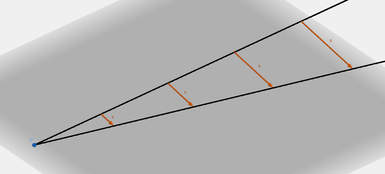
Another way to understand the Riemann tensor is through the geodesic deviation. Consider a point P in flat space from which go the geodesic lines:
and the separation between the geodesics (orange vector s) grows at a constant rate.
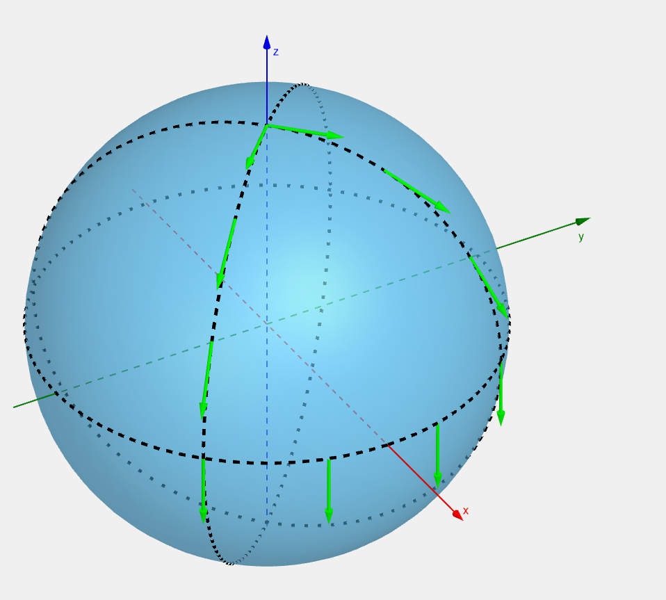
Now, consider the geodesics on a surface of a sphere:
we see that the geodesics accelerate away from each other and after crossing the equator, the accelerate back. Mathematically, it could be described as the covariant derivative of the separation vector s along a geodesic v:
∇vs∇vs=constant,=not constant, or:
∇v∇vs∇v∇vs=0,=0. Recall, from the covariant derivative chapter, we learned that the vector parallel transported along itself is geodesic:
∇vv=0. And the covariant covariant derivative of this along s is:
∇s∇vv∇s∇vv−∇v∇sv+∇v∇svR(s,v)v+∇v∇vs=0,=0,=0, where I have used the torsion-free property:
∇v∇sv=∇v∇vs. So the geodesic deviation is the output of the following Riemann tensor:
∇v∇vs=−R(s,v)v=R(v,s)v. When the Riemann tensor is zero, then there is no geodesic deviation. Implying that the space is flat.
Note: some sources may use a different sign convention:
∇v∇vs=R(s,v)v=−R(v,s)v. The second Bianchi identity is as follows:
(∇wR)(u,v)+(∇vR)(w,u)+(∇uR)(v,u)=0. or in component form:
Rσλαβ;γ+Rσλγα;β+Rσλβγ;α=0. The covariant derivative of the Riemann tensor is:
∇eγR=∇eγ(Rσλαβeσ⊗ϵλ⊗ϵα⊗ϵβ)=∇eγ(Rσλαβ)eσ⊗ϵλ⊗ϵα⊗ϵβ+Rσλαβ∇eγeσ⊗ϵλ⊗ϵα⊗ϵβ+Rσλαβeσ⊗∇eγϵλ⊗ϵα⊗ϵβ+Rσλαβeσ⊗ϵλ⊗∇eγϵα⊗ϵβ+Rσλαβeσ⊗ϵλ⊗ϵα⊗∇eγϵβ=Rσλαβ,γeσ⊗ϵλ⊗ϵα⊗ϵβ+RσλαβΓργσeρ⊗ϵλ⊗ϵα⊗ϵβ−RσλαβΓλγρeσ⊗ϵρ⊗ϵα⊗ϵβ−RσλαβΓαγρeσ⊗ϵλ⊗ϵρ⊗ϵβ−RσλαβΓβγρeσ⊗ϵλ⊗ϵα⊗ϵρ=Rσλαβ,γeσ⊗ϵλ⊗ϵα⊗ϵβ+RρλαβΓσγρeσ⊗ϵλ⊗ϵα⊗ϵβ−RσραβΓργλeσ⊗ϵλ⊗ϵα⊗ϵβ−RσλρβΓργαeσ⊗ϵλ⊗ϵα⊗ϵβ−RσλαρΓργβeσ⊗ϵλ⊗ϵα⊗ϵβ=(Rσλαβ,γ+RρλαβΓσγρ−RσραβΓργλ−RσλρβΓργα−RσλαρΓργβ)eσ⊗ϵλ⊗ϵα⊗ϵβ, or in component form:
Rσλαβ;γ=Rσλαβ,γ+RρλαβΓσγρ−RσραβΓργλ−RσλρβΓργα−RσλαρΓργβ. I won't prove the general version of this. I will however prove this in Riemann normal coordinates, where at a point p:
gμνgμνΓσμν=δμν,=δμν,=0, the covariant derivative (at point p) simplifies:
Rσλαβ;γ=Rσλαβ,γ, and the Riemann tensor components are:
Rσλαβ=Γσβλ,α−Γσαλ,β, then the covariant derivatives are:
Rσλαβ;γ=Γσβλ,αγ−Γσαλ,βγ. Substituting into the second Bianchi identity, we get:
Rσλαβ;γ+Rσλγα;β+Rσλβγ;α=Γσβλ,αγ−Γσαλ,βγ+Γσαλ,γβ−Γσγλ,αβ+Γσγλ,βα−Γσβλ,γα=Γσβλ,αγ−Γσβλ,γα+Γσαλ,γβ−Γσαλ,βγ+Γσγλ,βα−Γσγλ,αβ=0.