Back Geodesics and Christoffel Symbols Geodesic is the straightest and shortest path between two points in curved space. In flat space, this is straight line. In flat space, a straight path (geodesic) has zero acceleration (red arrows) if we travel along it at constant speed:
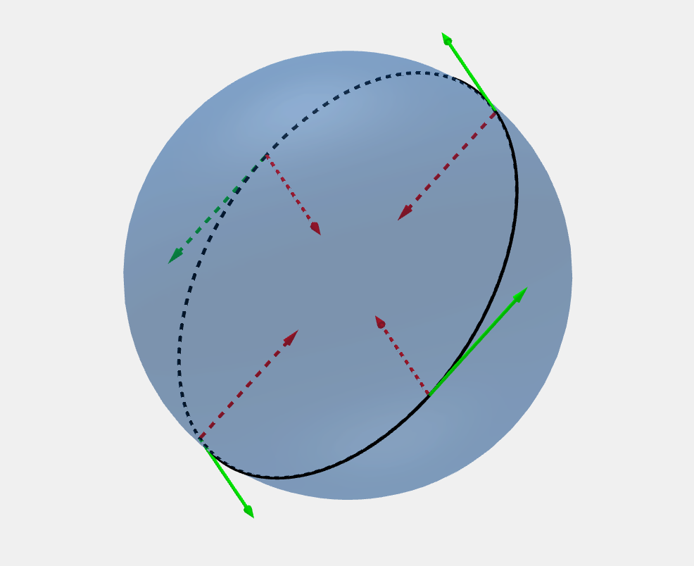
Non geodesic Geodesic For curved surfaces, there is not a straight path. However, there is a straightest possible path - the geodesic:
Non geodesic Geodesic The geodesic is a path where its acceleration (red vectors) is only in the normal components. This implies the tangential acceleration is zero.
We can write the acceleration (second derivative of extrinsic vector R \boldsymbol{R} R t t t n n n
d 2 R d λ 2 = ( d 2 R d λ 2 ) t + ( d 2 R d λ 2 ) n , \frac{d^2 \boldsymbol{R}}{d \lambda^2} = \left(\frac{d^2 \boldsymbol{R}}{d \lambda^2}\right)_t + \left(\frac{d^2 \boldsymbol{R}}{d \lambda^2}\right)_n, d λ 2 d 2 R = ( d λ 2 d 2 R ) t + ( d λ 2 d 2 R ) n , and the idea will be to set the tangential component equal to zero.
Calculating the second derivative:
d 2 R d λ 2 = d d λ ( d R μ d λ ∂ R ∂ R μ ) = d 2 R μ d λ 2 ∂ R ∂ R μ + d R μ d λ d d λ ( ∂ R ∂ R μ ) , \frac{d^2 \boldsymbol{R}}{d \lambda^2} = \frac{d}{d\lambda} \left(\frac{d R^{\mu}}{d \lambda} \frac{\partial \boldsymbol{R}}{\partial R^{\mu}}\right) = \frac{d^2 R^{\mu}}{d \lambda^2} \frac{\partial \boldsymbol{R}}{\partial R^{\mu}} + \frac{d R^{\mu}}{d \lambda} \frac{d}{d\lambda} \left(\frac{\partial \boldsymbol{R}}{\partial R^{\mu}}\right), d λ 2 d 2 R = d λ d ( d λ d R μ ∂ R μ ∂ R ) = d λ 2 d 2 R μ ∂ R μ ∂ R + d λ d R μ d λ d ( ∂ R μ ∂ R ) , we can expand the derivative operator:
d d λ = d R μ d λ ∂ ∂ R μ , \frac{d}{d \lambda} = \frac{d R^{\mu}}{d \lambda} \frac{\partial}{\partial R^{\mu}}, d λ d = d λ d R μ ∂ R μ ∂ , substituting it back:
d 2 R d λ 2 = d 2 R μ d λ 2 ∂ R ∂ R μ + d R μ d λ d R ν d λ ∂ ∂ R ν ( ∂ R ∂ R μ ) = d 2 R μ d λ 2 ∂ R ∂ R μ + d R μ d λ d R ν d λ ∂ 2 R ∂ R μ ∂ R ν , \begin{align*} \frac{d^2 \boldsymbol{R}}{d \lambda^2} &= \frac{d^2 R^{\mu}}{d \lambda^2} \frac{\partial \boldsymbol{R}}{\partial R^{\mu}} + \frac{d R^{\mu}}{d \lambda} \frac{d R^{\nu}}{d \lambda} \frac{\partial}{\partial R^{\nu}} \left(\frac{\partial \boldsymbol{R}}{\partial R^{\mu}}\right) \\ &= \frac{d^2 R^{\mu}}{d \lambda^2} \frac{\partial \boldsymbol{R}}{\partial R^{\mu}} + \frac{d R^{\mu}}{d \lambda} \frac{d R^{\nu}}{d \lambda} \frac{\partial^2 \boldsymbol{R}}{\partial R^{\mu} \partial R^{\nu}}, \end{align*} d λ 2 d 2 R = d λ 2 d 2 R μ ∂ R μ ∂ R + d λ d R μ d λ d R ν ∂ R ν ∂ ( ∂ R μ ∂ R ) = d λ 2 d 2 R μ ∂ R μ ∂ R + d λ d R μ d λ d R ν ∂ R μ ∂ R ν ∂ 2 R , here, R μ R^{\mu} R μ R ν R^{\nu} R ν θ \theta θ ϕ \phi ϕ
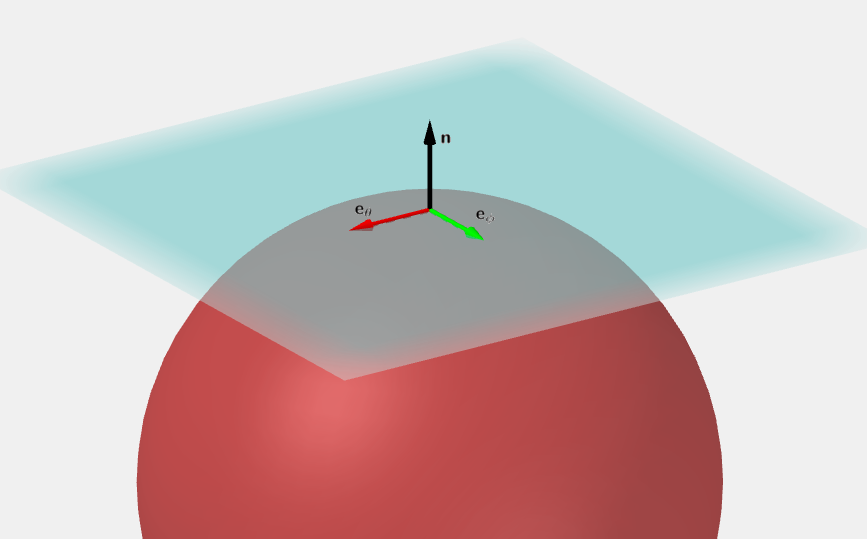
To make sense of the second partial derivative, consider the tangent plane of a sphere:
In the 2D surface, the second partial derivative will be three dimensional (with non zero normal components). We don't know the components, so we will invent them:
∂ 2 R ∂ R μ ∂ R ν = Γ θ μ ν e θ + Γ ϕ μ ν e ϕ + L μ ν n ^ , \frac{\partial^2 \boldsymbol{R}}{\partial R^{\mu} \partial R^{\nu}} = \Gamma^{\theta}{}_{\mu \nu} \boldsymbol{e_{\theta}} + \Gamma^{\phi}{}_{\mu \nu} \boldsymbol{e_{\phi}} + L_{\mu \nu} \boldsymbol{\hat{n}}, ∂ R μ ∂ R ν ∂ 2 R = Γ θ μν e θ + Γ ϕ μν e ϕ + L μν n ^ , or generally for any coordinates and any dimensions:
∂ 2 R ∂ R μ ∂ R ν = Γ σ μ ν e σ + L μ ν n ^ = Γ σ μ ν ∂ R ∂ R σ + L μ ν n ^ , \begin{align*} \frac{\partial^2 \boldsymbol{R}}{\partial R^{\mu} \partial R^{\nu}} &= \Gamma^{\sigma}{}_{\mu \nu} \boldsymbol{e_{\sigma}} + L_{\mu \nu} \boldsymbol{\hat{n}} \\ &= \Gamma^{\sigma}{}_{\mu \nu} \frac{\partial \boldsymbol{R}}{\partial R^{\sigma}} + L_{\mu \nu} \boldsymbol{\hat{n}}, \end{align*} ∂ R μ ∂ R ν ∂ 2 R = Γ σ μν e σ + L μν n ^ = Γ σ μν ∂ R σ ∂ R + L μν n ^ , where Γ σ μ ν \Gamma^{\sigma}{}_{\mu \nu} Γ σ μν L μ ν L_{\mu \nu} L μν
Substituting into the equation for acceleration:
d 2 R d λ 2 = d 2 R μ d λ 2 ∂ R ∂ R μ + d R μ d λ d R ν d λ ( Γ σ μ ν ∂ R ∂ R σ + L μ ν n ^ ) = d 2 R σ d λ 2 ∂ R ∂ R σ + Γ σ μ ν d R μ d λ d R ν d λ ∂ R ∂ R σ + L μ ν d R μ d λ d R ν d λ n ^ = ( d 2 R σ d λ 2 + Γ σ μ ν d R μ d λ d R ν d λ ) ∂ R ∂ R σ + L μ ν d R μ d λ d R ν d λ n ^ . \begin{align*} \frac{d^2 \boldsymbol{R}}{d \lambda^2} &= \frac{d^2 R^{\mu}}{d \lambda^2} \frac{\partial \boldsymbol{R}}{\partial R^{\mu}} + \frac{d R^{\mu}}{d \lambda} \frac{d R^{\nu}}{d \lambda} \left(\Gamma^{\sigma}{}_{\mu \nu} \frac{\partial \boldsymbol{R}}{\partial R^{\sigma}} + L_{\mu \nu} \boldsymbol{\hat{n}}\right) \\ &= \frac{d^2 R^{\sigma}}{d \lambda^2} \frac{\partial \boldsymbol{R}}{\partial R^{\sigma}} + \Gamma^{\sigma}{}_{\mu \nu} \frac{d R^{\mu}}{d \lambda} \frac{d R^{\nu}}{d \lambda} \frac{\partial \boldsymbol{R}}{\partial R^{\sigma}} + L_{\mu \nu} \frac{d R^{\mu}}{d \lambda} \frac{d R^{\nu}}{d \lambda} \boldsymbol{\hat{n}} \\ &= \left(\frac{d^2 R^{\sigma}}{d \lambda^2} + \Gamma^{\sigma}{}_{\mu \nu} \frac{d R^{\mu}}{d \lambda} \frac{d R^{\nu}}{d \lambda}\right) \frac{\partial \boldsymbol{R}}{\partial R^{\sigma}} + L_{\mu \nu} \frac{d R^{\mu}}{d \lambda} \frac{d R^{\nu}}{d \lambda} \boldsymbol{\hat{n}}. \\ \end{align*} d λ 2 d 2 R = d λ 2 d 2 R μ ∂ R μ ∂ R + d λ d R μ d λ d R ν ( Γ σ μν ∂ R σ ∂ R + L μν n ^ ) = d λ 2 d 2 R σ ∂ R σ ∂ R + Γ σ μν d λ d R μ d λ d R ν ∂ R σ ∂ R + L μν d λ d R μ d λ d R ν n ^ = ( d λ 2 d 2 R σ + Γ σ μν d λ d R μ d λ d R ν ) ∂ R σ ∂ R + L μν d λ d R μ d λ d R ν n ^ . We now have the tangential and normal components separated. The geodesics have zero tangential acceleration:
( d 2 R σ d λ 2 + Γ σ μ ν d R μ d λ d R ν d λ ) ∂ R ∂ R σ = 0 , d 2 R σ d λ 2 + Γ σ μ ν d R μ d λ d R ν d λ = 0 , \begin{align*} \left(\frac{d^2 R^{\sigma}}{d \lambda^2} + \Gamma^{\sigma}{}_{\mu \nu} \frac{d R^{\mu}}{d \lambda} \frac{d R^{\nu}}{d \lambda}\right) \frac{\partial \boldsymbol{R}}{\partial R^{\sigma}} &= \boldsymbol{0}, \\ \frac{d^2 R^{\sigma}}{d \lambda^2} + \Gamma^{\sigma}{}_{\mu \nu} \frac{d R^{\mu}}{d \lambda} \frac{d R^{\nu}}{d \lambda} &= 0, \end{align*} ( d λ 2 d 2 R σ + Γ σ μν d λ d R μ d λ d R ν ) ∂ R σ ∂ R d λ 2 d 2 R σ + Γ σ μν d λ d R μ d λ d R ν = 0 , = 0 , the second equation is a set of equations that each of σ \sigma σ
Christoffel symbols can be calculated by using the fact that the dot product of perpendicular vector is zero (by definition, the normal vector is perpendicular to the tangent vectors):
∂ 2 R ∂ R μ ∂ R ν = Γ σ μ ν ∂ R ∂ R σ + L μ ν n ^ , ∂ 2 R ∂ R μ ∂ R ν ⋅ ∂ R ∂ R λ = ( Γ σ μ ν ∂ R ∂ R σ + L μ ν n ^ ) ⋅ ∂ R ∂ R λ = Γ σ μ ν ∂ R ∂ R σ ⋅ ∂ R ∂ R λ + L μ ν n ^ ⋅ ∂ R ∂ R λ = Γ σ μ ν g σ λ , Γ λ μ ν = ∂ 2 R ∂ R μ ∂ R ν ⋅ ∂ R ∂ R λ = ∂ e μ ∂ R ν ⋅ e λ , Γ λ μ ν = ∂ 2 R ∂ R μ ∂ R ν ⋅ ∂ R ∂ R σ g σ λ = ∂ e μ ∂ R ν ⋅ e σ g σ λ , \begin{align*} \frac{\partial^2 \boldsymbol{R}}{\partial R^{\mu} \partial R^{\nu}} &= \Gamma^{\sigma}{}_{\mu \nu} \frac{\partial \boldsymbol{R}}{\partial R^{\sigma}} + L_{\mu \nu} \boldsymbol{\hat{n}}, \\ \frac{\partial^2 \boldsymbol{R}}{\partial R^{\mu} \partial R^{\nu}} \cdot \frac{\partial \boldsymbol{R}}{\partial R^{\lambda}} &= \left(\Gamma^{\sigma}{}_{\mu \nu} \frac{\partial \boldsymbol{R}}{\partial R^{\sigma}} + L_{\mu \nu} \boldsymbol{\hat{n}}\right) \cdot \frac{\partial \boldsymbol{R}}{\partial R^{\lambda}} \\ &= \Gamma^{\sigma}{}_{\mu \nu} \frac{\partial \boldsymbol{R}}{\partial R^{\sigma}} \cdot \frac{\partial \boldsymbol{R}}{\partial R^{\lambda}} + L_{\mu \nu} \boldsymbol{\hat{n}} \cdot \frac{\partial \boldsymbol{R}}{\partial R^{\lambda}} \\ &= \Gamma^{\sigma}{}_{\mu \nu} g_{\sigma \lambda}, \\ \Gamma_{\lambda \mu \nu} &= \frac{\partial^2 \boldsymbol{R}}{\partial R^{\mu} \partial R^{\nu}} \cdot \frac{\partial \boldsymbol{R}}{\partial R^{\lambda}} = \frac{\partial \boldsymbol{e_{\mu}}}{\partial R^{\nu}} \cdot \boldsymbol{e_{\lambda}}, \\ \Gamma^{\lambda}{}_{\mu \nu} &= \frac{\partial^2 \boldsymbol{R}}{\partial R^{\mu} \partial R^{\nu}} \cdot \frac{\partial \boldsymbol{R}}{\partial R^{\sigma}} g^{\sigma \lambda} = \frac{\partial \boldsymbol{e_{\mu}}}{\partial R^{\nu}} \cdot \boldsymbol{e_{\sigma}} g^{\sigma \lambda}, \end{align*} ∂ R μ ∂ R ν ∂ 2 R ∂ R μ ∂ R ν ∂ 2 R ⋅ ∂ R λ ∂ R Γ λ μν Γ λ μν = Γ σ μν ∂ R σ ∂ R + L μν n ^ , = ( Γ σ μν ∂ R σ ∂ R + L μν n ^ ) ⋅ ∂ R λ ∂ R = Γ σ μν ∂ R σ ∂ R ⋅ ∂ R λ ∂ R + L μν n ^ ⋅ ∂ R λ ∂ R = Γ σ μν g σλ , = ∂ R μ ∂ R ν ∂ 2 R ⋅ ∂ R λ ∂ R = ∂ R ν ∂ e μ ⋅ e λ , = ∂ R μ ∂ R ν ∂ 2 R ⋅ ∂ R σ ∂ R g σλ = ∂ R ν ∂ e μ ⋅ e σ g σλ , where Γ λ μ ν \Gamma_{\lambda \mu \nu} Γ λ μν Γ λ μ ν \Gamma^{\lambda}{}_{\mu \nu} Γ λ μν R \boldsymbol{R} R
Similarly, we can solve for the second fundamental form:
∂ 2 R ∂ R μ ∂ R ν = Γ σ μ ν ∂ R ∂ R σ + L μ ν n ^ , ∂ 2 R ∂ R μ ∂ R ν ⋅ n ^ = ( Γ σ μ ν ∂ R ∂ R σ + L μ ν n ^ ) ⋅ n ^ = Γ σ μ ν ∂ R ∂ R σ ⋅ n ^ + L μ ν n ^ ⋅ n ^ = L μ ν . \begin{align*} \frac{\partial^2 \boldsymbol{R}}{\partial R^{\mu} \partial R^{\nu}} &= \Gamma^{\sigma}{}_{\mu \nu} \frac{\partial \boldsymbol{R}}{\partial R^{\sigma}} + L_{\mu \nu} \boldsymbol{\hat{n}}, \\ \frac{\partial^2 \boldsymbol{R}}{\partial R^{\mu} \partial R^{\nu}} \cdot \boldsymbol{\hat{n}} &= \left(\Gamma^{\sigma}{}_{\mu \nu} \frac{\partial \boldsymbol{R}}{\partial R^{\sigma}} + L_{\mu \nu} \boldsymbol{\hat{n}}\right) \cdot \boldsymbol{\hat{n}} \\ &= \Gamma^{\sigma}{}_{\mu \nu} \frac{\partial \boldsymbol{R}}{\partial R^{\sigma}} \cdot \boldsymbol{\hat{n}} + L_{\mu \nu} \boldsymbol{\hat{n}} \cdot \boldsymbol{\hat{n}} \\ &= L_{\mu \nu}. \end{align*} ∂ R μ ∂ R ν ∂ 2 R ∂ R μ ∂ R ν ∂ 2 R ⋅ n ^ = Γ σ μν ∂ R σ ∂ R + L μν n ^ , = ( Γ σ μν ∂ R σ ∂ R + L μν n ^ ) ⋅ n ^ = Γ σ μν ∂ R σ ∂ R ⋅ n ^ + L μν n ^ ⋅ n ^ = L μν . The normal vector may also be given by cross product of the basis vectors (divided by its length to have length equal to one):
L μ ν = ∂ e μ ∂ R ν ⋅ e μ × e μ ∣ e μ × e μ ∣ . L_{\mu \nu} = \frac{\partial \boldsymbol{e_{\mu}}}{\partial R^{\nu}} \cdot \frac{\boldsymbol{e_{\mu}} \times \boldsymbol{e_{\mu}}}{|\boldsymbol{e_{\mu}} \times \boldsymbol{e_{\mu}}|}. L μν = ∂ R ν ∂ e μ ⋅ ∣ e μ × e μ ∣ e μ × e μ . Since the order of partial differentiation does not matter, we can prove the following symmetry:
Γ λ μ ν = ∂ 2 R ∂ R μ ∂ R ν ⋅ ∂ R ∂ R λ = ∂ 2 R ∂ R ν ∂ R μ ⋅ ∂ R ∂ R λ = Γ λ ν μ , Γ λ μ ν = ∂ 2 R ∂ R μ ∂ R ν ⋅ ∂ R ∂ R σ g σ λ = ∂ 2 R ∂ R ν ∂ R μ ⋅ ∂ R ∂ R σ g σ λ = Γ λ ν μ . \begin{align*} \Gamma_{\lambda \mu \nu} &= \frac{\partial^2 \boldsymbol{R}}{\partial R^{\mu} \partial R^{\nu}} \cdot \frac{\partial \boldsymbol{R}}{\partial R^{\lambda}} = \frac{\partial^2 \boldsymbol{R}}{\partial R^{\nu} \partial R^{\mu}} \cdot \frac{\partial \boldsymbol{R}}{\partial R^{\lambda}} = \Gamma_{\lambda \nu \mu}, \\ \Gamma^{\lambda}{}_{\mu \nu} &= \frac{\partial^2 \boldsymbol{R}}{\partial R^{\mu} \partial R^{\nu}} \cdot \frac{\partial \boldsymbol{R}}{\partial R^{\sigma}} g^{\sigma \lambda} = \frac{\partial^2 \boldsymbol{R}}{\partial R^{\nu} \partial R^{\mu}} \cdot \frac{\partial \boldsymbol{R}}{\partial R^{\sigma}} g^{\sigma \lambda} = \Gamma^{\lambda}{}_{\nu \mu}. \end{align*} Γ λ μν Γ λ μν = ∂ R μ ∂ R ν ∂ 2 R ⋅ ∂ R λ ∂ R = ∂ R ν ∂ R μ ∂ 2 R ⋅ ∂ R λ ∂ R = Γ λ νμ , = ∂ R μ ∂ R ν ∂ 2 R ⋅ ∂ R σ ∂ R g σλ = ∂ R ν ∂ R μ ∂ 2 R ⋅ ∂ R σ ∂ R g σλ = Γ λ νμ . The Christoffel symbols are not a tensor. They do not transform under the change of coordinates like tensors:
Γ ~ σ μ ν ≠ ∂ x ~ σ ∂ x α ∂ x β ∂ x ~ μ ∂ x γ ∂ x ~ ν Γ β γ α . \tilde{\Gamma}^{\sigma}{}_{\mu \nu} \neq \frac{\partial \tilde{x}^{\sigma}}{\partial x^{\alpha}} \frac{\partial x^{\beta}}{\partial \tilde{x}^{\mu}} \frac{\partial x^{\gamma}}{\partial \tilde{x}^{\nu}} \Gamma^{\alpha}_{\beta \gamma}. Γ ~ σ μν = ∂ x α ∂ x ~ σ ∂ x ~ μ ∂ x β ∂ x ~ ν ∂ x γ Γ β γ α . This will be proven in the next chapter .
Consider the 2D Cartesian coordinates in flat plane. We know that the basis vectors don't change, implying:
∂ e μ ∂ R ν = 0 , Γ λ μ ν = 0 ⋅ e σ g σ λ = 0. \begin{align*} \frac{\partial \boldsymbol{e_{\mu}}}{\partial R^{\nu}} &= \boldsymbol{0}, \\ \Gamma^{\lambda}{}_{\mu \nu} &= \boldsymbol{0} \cdot \boldsymbol{e_{\sigma}} g^{\sigma \lambda} = 0. \end{align*} ∂ R ν ∂ e μ Γ λ μν = 0 , = 0 ⋅ e σ g σλ = 0. This simplifies the geodesic equations:
d 2 R σ d λ 2 = 0 , \frac{d^2 R^{\sigma}}{d \lambda^2} = 0, d λ 2 d 2 R σ = 0 , implying:
R σ = C σ λ + R 0 σ , R^{\sigma} = C_{\sigma} \lambda + R^{\sigma}_0, R σ = C σ λ + R 0 σ , where C σ C_{\sigma} C σ R 0 σ R^{\sigma}_0 R 0 σ C σ C_{\sigma} C σ R 0 σ R^{\sigma}_0 R 0 σ
However, when we consider the 2D polar coordinates where:
x = r cos θ , y = r sin θ , r = x 2 + y 2 , θ = tan − 1 ( y x ) , \begin{align*} x &= r \cos \theta, \\ y &= r \sin \theta, \\ r &= \sqrt{x^2 + y^2}, \\ \theta &= \tan^{-1} \left(\frac{y}{x}\right), \end{align*} x y r θ = r cos θ , = r sin θ , = x 2 + y 2 , = tan − 1 ( x y ) , where the metric tensor and its inverse are equal to:
g ~ μ ν = [ 1 0 0 r 2 ] , g ~ μ ν = [ 1 0 0 1 r 2 ] . \begin{align*} \tilde{g}_{\mu \nu} &= \begin{bmatrix} 1 & 0 \\ 0 & r^2 \end{bmatrix}, \\ \tilde{g}^{\mu \nu} &= \begin{bmatrix} 1 & 0 \\ 0 & \frac{1}{r^2} \end{bmatrix}. \end{align*} g ~ μν g ~ μν = [ 1 0 0 r 2 ] , = [ 1 0 0 r 2 1 ] . The Jacobian is:
∂ x ∂ r = cos θ , ∂ x ∂ r = − r sin θ , ∂ y ∂ r = sin θ , ∂ y ∂ r = r cos θ , \begin{align*} \frac{\partial x}{\partial r} &= \cos \theta, & \frac{\partial x}{\partial r} &= -r \sin \theta, \\ \frac{\partial y}{\partial r} &= \sin \theta, & \frac{\partial y}{\partial r} &= r \cos \theta, \end{align*} ∂ r ∂ x ∂ r ∂ y = cos θ , = sin θ , ∂ r ∂ x ∂ r ∂ y = − r sin θ , = r cos θ , and the inverse Jacobian:
∂ r ∂ x = x x 2 + y 2 = cos θ , ∂ r ∂ y = y x 2 + y 2 = sin θ , ∂ θ ∂ x = − y x 2 + y 2 = − sin θ r , ∂ θ ∂ y = x x 2 + y 2 = cos θ r . \begin{align*} \frac{\partial r}{\partial x} &= \frac{x}{\sqrt{x^2 + y^2}} = \cos \theta, & \frac{\partial r}{\partial y} &= \frac{y}{\sqrt{x^2 + y^2}} = \sin \theta, \\ \frac{\partial \theta}{\partial x} &= -\frac{y}{x^2 + y^2} = - \frac{\sin \theta}{r}, & \frac{\partial \theta}{\partial y} &= \frac{x}{x^2 + y^2} = \frac{\cos \theta}{r}. \end{align*} ∂ x ∂ r ∂ x ∂ θ = x 2 + y 2 x = cos θ , = − x 2 + y 2 y = − r sin θ , ∂ y ∂ r ∂ y ∂ θ = x 2 + y 2 y = sin θ , = x 2 + y 2 x = r cos θ . The basis vectors transform covariantly:
e ~ μ = ∂ x ν ∂ x ~ μ e ν , \boldsymbol{\tilde{e}_{\mu}} = \frac{\partial x^{\nu}}{\partial \tilde{x}^{\mu}} \boldsymbol{e_{\nu}}, e ~ μ = ∂ x ~ μ ∂ x ν e ν , where the individual basis vectors are as follows:
e ~ r = ∂ x ∂ r e x + ∂ y ∂ r e y = cos θ e x + sin θ e y , e ~ θ = ∂ x ∂ θ e x + ∂ y ∂ θ e y = − r sin θ e x + r cos θ e y . \begin{align*} \boldsymbol{\tilde{e}_r} &= \frac{\partial x}{\partial r} \boldsymbol{e_x} + \frac{\partial y}{\partial r} \boldsymbol{e_y} \\ &= \cos \theta \boldsymbol{e_x} + \sin \theta \boldsymbol{e_y}, \\ \boldsymbol{\tilde{e}_{\theta}} &= \frac{\partial x}{\partial \theta} \boldsymbol{e_x} + \frac{\partial y}{\partial \theta} \boldsymbol{e_y} \\ &= - r \sin \theta \boldsymbol{e_x} + r \cos \theta \boldsymbol{e_y}. \end{align*} e ~ r e ~ θ = ∂ r ∂ x e x + ∂ r ∂ y e y = cos θ e x + sin θ e y , = ∂ θ ∂ x e x + ∂ θ ∂ y e y = − r sin θ e x + r cos θ e y . To compute the Christoffel symbols, we need partial derivatives of the basis vectors:
∂ e ~ r ∂ r = 0 , ∂ e ~ θ ∂ θ = − r cos θ e x − r sin θ e y , ∂ e ~ θ ∂ r = ∂ e ~ r ∂ θ = − sin θ e x + cos θ e y . \begin{align*} \frac{\partial \boldsymbol{\tilde{e}_r}}{\partial r} &= \boldsymbol{0}, \\ \frac{\partial \boldsymbol{\tilde{e}_\theta}}{\partial \theta} &= -r \cos \theta \boldsymbol{e_x} - r \sin \theta \boldsymbol{e_y}, \\ \frac{\partial \boldsymbol{\tilde{e}_{\theta}}}{\partial r} = \frac{\partial \boldsymbol{\tilde{e}_r}}{\partial \theta} &= -\sin \theta \boldsymbol{e_x} + \cos \theta \boldsymbol{e_y}. \end{align*} ∂ r ∂ e ~ r ∂ θ ∂ e ~ θ ∂ r ∂ e ~ θ = ∂ θ ∂ e ~ r = 0 , = − r cos θ e x − r sin θ e y , = − sin θ e x + cos θ e y . The Christoffel symbols are equal to:
Γ μ ν λ = ∂ e ~ μ ∂ x ~ ν ⋅ e ~ σ g ~ σ λ , Γ μ ν r = ∂ e ~ μ ∂ x ~ ν ⋅ e ~ r g ~ r r , Γ μ ν θ = ∂ e ~ μ ∂ x ~ ν ⋅ e ~ θ g ~ θ θ , \begin{align*} \Gamma^{\lambda}_{\mu \nu} &= \frac{\partial \boldsymbol{\tilde{e}_{\mu}}}{\partial \tilde{x}^{\nu}} \cdot \boldsymbol{\tilde{e}_{\sigma}} \tilde{g}^{\sigma \lambda}, \\[3ex] \Gamma^r_{\mu \nu} &= \frac{\partial \boldsymbol{\tilde{e}_{\mu}}}{\partial \tilde{x}^{\nu}} \cdot \boldsymbol{\tilde{e}_r} \tilde{g}^{r r}, \\ \Gamma^{\theta}_{\mu \nu} &= \frac{\partial \boldsymbol{\tilde{e}_{\mu}}}{\partial \tilde{x}^{\nu}} \cdot \boldsymbol{\tilde{e}_{\theta}} \tilde{g}^{\theta \theta}, \end{align*} Γ μν λ Γ μν r Γ μν θ = ∂ x ~ ν ∂ e ~ μ ⋅ e ~ σ g ~ σλ , = ∂ x ~ ν ∂ e ~ μ ⋅ e ~ r g ~ rr , = ∂ x ~ ν ∂ e ~ μ ⋅ e ~ θ g ~ θθ , and the individual components:
Γ r r r = [ 0 0 ] ⋅ [ cos θ sin θ ] = 0 , Γ r θ r = Γ θ r r = [ − sin θ cos θ ] ⋅ [ cos θ sin θ ] = − sin θ cos θ + sin θ cos θ = 0 , Γ θ θ r = [ − r cos θ − r sin θ ] ⋅ [ cos θ sin θ ] = − r cos 2 θ + − r sin 2 θ = − r , Γ r r θ = [ 0 0 ] ⋅ [ − r sin θ r cos θ ] 1 r 2 = 0 , Γ r θ θ = Γ θ r θ = [ − sin θ cos θ ] ⋅ [ − r sin θ r cos θ ] 1 r 2 = ( r sin 2 θ + r cos 2 θ ) 1 r 2 = 1 r . Γ θ θ θ = [ − r cos θ − r sin θ ] ⋅ [ − r sin θ r cos θ ] = r 2 sin θ cos θ − r 2 sin θ cos θ = 0. \begin{align*} \Gamma^r_{rr} &= \begin{bmatrix} 0 \\ 0 \end{bmatrix} \cdot \begin{bmatrix} \cos \theta \\ \sin \theta \end{bmatrix} \\ &= 0, \\ \Gamma^r_{r\theta} = \Gamma^r_{\theta r} &= \begin{bmatrix} -\sin \theta \\ \cos \theta \end{bmatrix} \cdot \begin{bmatrix} \cos \theta \\ \sin \theta \end{bmatrix} \\ &= - \sin \theta \cos \theta + \sin \theta \cos \theta \\ &= 0, \\ \Gamma^r_{\theta \theta} &= \begin{bmatrix} -r \cos \theta \\ -r \sin \theta \end{bmatrix} \cdot \begin{bmatrix} \cos \theta \\ \sin \theta \end{bmatrix} \\ &= -r \cos^2 \theta + -r \sin^2 \theta \\ &= -r, \\ \Gamma^{\theta}_{rr} &= \begin{bmatrix} 0 \\ 0 \end{bmatrix} \cdot \begin{bmatrix} - r \sin \theta \\ r \cos \theta \end{bmatrix} \frac{1}{r^2} \\ &= 0, \\ \Gamma^{\theta}_{r \theta} = \Gamma^{\theta}_{\theta r} &= \begin{bmatrix} - \sin \theta \\ \cos \theta \\ \end{bmatrix} \cdot \begin{bmatrix} - r \sin \theta \\ r \cos \theta \end{bmatrix} \frac{1}{r^2} \\ &= (r \sin^2 \theta + r \cos^2 \theta) \frac{1}{r^2} \\ &= \frac{1}{r}. \\ \Gamma^{\theta}_{\theta \theta} &= \begin{bmatrix} -r \cos \theta \\ -r \sin \theta \end{bmatrix} \cdot \begin{bmatrix} -r \sin \theta \\ r \cos \theta \end{bmatrix} \\ &= r^2 \sin \theta \cos \theta - r^2 \sin \theta \cos \theta \\ &= 0. \end{align*} Γ rr r Γ r θ r = Γ θ r r Γ θθ r Γ rr θ Γ r θ θ = Γ θ r θ Γ θθ θ = [ 0 0 ] ⋅ [ cos θ sin θ ] = 0 , = [ − sin θ cos θ ] ⋅ [ cos θ sin θ ] = − sin θ cos θ + sin θ cos θ = 0 , = [ − r cos θ − r sin θ ] ⋅ [ cos θ sin θ ] = − r cos 2 θ + − r sin 2 θ = − r , = [ 0 0 ] ⋅ [ − r sin θ r cos θ ] r 2 1 = 0 , = [ − sin θ cos θ ] ⋅ [ − r sin θ r cos θ ] r 2 1 = ( r sin 2 θ + r cos 2 θ ) r 2 1 = r 1 . = [ − r cos θ − r sin θ ] ⋅ [ − r sin θ r cos θ ] = r 2 sin θ cos θ − r 2 sin θ cos θ = 0. where the dot product between column vectors is the Cartesian dot product.
The only nonzero Christoffel symbols are:
Γ θ θ r = − r , Γ r θ θ = Γ θ r θ = 1 r , \begin{align*} \Gamma^r_{\theta \theta} &= -r, \\ \Gamma^{\theta}_{r \theta} = \Gamma^{\theta}_{\theta r} &= \frac{1}{r}, \end{align*} Γ θθ r Γ r θ θ = Γ θ r θ = − r , = r 1 , and the geodesic equations are as follows:
d 2 r d λ 2 − r ( d θ d λ ) 2 = 0 , d 2 θ d λ 2 + 2 r d r d λ d θ d λ = 0. \begin{align*} \frac{d^2 r}{d \lambda^2} - r \left(\frac{d \theta}{d \lambda}\right)^2 &= 0, \\ \frac{d^2 \theta}{d \lambda^2} + \frac{2}{r} \frac{d r}{d \lambda} \frac{d \theta}{d \lambda} &= 0. \end{align*} d λ 2 d 2 r − r ( d λ d θ ) 2 d λ 2 d 2 θ + r 2 d λ d r d λ d θ = 0 , = 0. I will not be solving these. I will, however, the scenario where θ = θ 0 ⟹ d 2 θ d λ 2 = d θ d λ = 0 \theta = \theta_0 \implies \frac{d^2 \theta}{d\lambda^2} = \frac{d\theta}{d\lambda} = 0 θ = θ 0 ⟹ d λ 2 d 2 θ = d λ d θ = 0
d 2 r d λ 2 = 0 , r = v ∥ λ + r 0 , \begin{align*} \frac{d^2 r}{d\lambda^2} &= 0, \\ r &= v_{\parallel} \lambda + r_0, \end{align*} d λ 2 d 2 r r = 0 , = v ∥ λ + r 0 , where v ∥ v_{\parallel} v ∥ r 0 r_0 r 0 r r r
In the metric tensor , we derived the intrinsic basis vectors and the metric tensor:
e ˉ θ = r cos θ cos ϕ e x + r cos θ sin ϕ e y − r sin θ e z , e ˉ ϕ = − r sin θ sin ϕ e x + r sin θ cos ϕ e y , g ˉ μ ν = [ r 2 0 0 r 2 sin 2 θ ] , \begin{align*} \boldsymbol{\bar{e}_{\theta}} &= r \cos \theta \cos \phi \boldsymbol{e_x} + r \cos \theta \sin \phi \boldsymbol{e_y} - r \sin \theta \boldsymbol{e_z}, \\ \boldsymbol{\bar{e}_{\phi}} &= -r \sin \theta \sin \phi \boldsymbol{e_x} + r \sin \theta \cos \phi \boldsymbol{e_y}, \\ \bar{g}_{\mu \nu} &= \begin{bmatrix} r^2 & 0 \\ 0 & r^2 \sin^2 \theta \end{bmatrix}, \end{align*} e ˉ θ e ˉ ϕ g ˉ μν = r cos θ cos ϕ e x + r cos θ sin ϕ e y − r sin θ e z , = − r sin θ sin ϕ e x + r sin θ cos ϕ e y , = [ r 2 0 0 r 2 sin 2 θ ] , and the inverse metric tensor is equal to:
g ˉ μ ν = [ 1 r 2 0 0 1 r 2 sin 2 θ ] . \begin{align*} \bar{g}^{\mu \nu} &= \begin{bmatrix} \frac{1}{r^2} & 0 \\ 0 & \frac{1}{r^2 \sin^2 \theta} \end{bmatrix}. \end{align*} g ˉ μν = [ r 2 1 0 0 r 2 s i n 2 θ 1 ] . The partial derivatives of the basis vectors are equal to:
∂ e ˉ θ ∂ θ = − r sin θ cos ϕ e x − r sin θ sin ϕ e y − r cos θ e z , ∂ e ˉ ϕ ∂ ϕ = − r sin θ cos ϕ e x − r sin θ sin ϕ e y , ∂ e ˉ ϕ ∂ θ = ∂ e ˉ θ ∂ ϕ = − r cos θ sin ϕ e x + r cos θ cos ϕ e y . \begin{align*} \frac{\partial \boldsymbol{\bar{e}_{\theta}}}{\partial \theta} &= -r \sin \theta \cos \phi \boldsymbol{e_x} - r \sin \theta \sin \phi \boldsymbol{e_y} - r \cos \theta \boldsymbol{e_z}, \\ \frac{\partial \boldsymbol{\bar{e}_{\phi}}}{\partial \phi} &= -r \sin \theta \cos \phi \boldsymbol{e_x} - r \sin \theta \sin \phi \boldsymbol{e_y}, \\ \frac{\partial \boldsymbol{\bar{e}_{\phi}}}{\partial \theta} = \frac{\partial \boldsymbol{\bar{e}_{\theta}}}{\partial \phi} &= -r \cos \theta \sin \phi \boldsymbol{e_x} + r \cos \theta \cos \phi \boldsymbol{e_y}. \end{align*} ∂ θ ∂ e ˉ θ ∂ ϕ ∂ e ˉ ϕ ∂ θ ∂ e ˉ ϕ = ∂ ϕ ∂ e ˉ θ = − r sin θ cos ϕ e x − r sin θ sin ϕ e y − r cos θ e z , = − r sin θ cos ϕ e x − r sin θ sin ϕ e y , = − r cos θ sin ϕ e x + r cos θ cos ϕ e y . Since the metric tensor and its inverse is diagonal, the Christoffel symbols simplify:
Γ θ μ ν = ∂ e ˉ μ ∂ R ν ⋅ e ˉ θ g θ θ , Γ ϕ μ ν = ∂ e ˉ μ ∂ R ν ⋅ e ˉ ϕ g ϕ ϕ . \begin{align*} \Gamma^{\theta}{}_{\mu \nu} = \frac{\partial \boldsymbol{\bar{e}_{\mu}}}{\partial R^{\nu}} \cdot \boldsymbol{\bar{e}_{\theta}} g^{\theta \theta}, \\ \Gamma^{\phi}{}_{\mu \nu} = \frac{\partial \boldsymbol{\bar{e}_{\mu}}}{\partial R^{\nu}} \cdot \boldsymbol{\bar{e}_{\phi}} g^{\phi \phi}. \end{align*} Γ θ μν = ∂ R ν ∂ e ˉ μ ⋅ e ˉ θ g θθ , Γ ϕ μν = ∂ R ν ∂ e ˉ μ ⋅ e ˉ ϕ g ϕϕ . The individual Christoffel symbols are equal to:
Γ θ θ θ = [ − r sin θ cos ϕ − r sin θ sin ϕ − r cos θ ] ⋅ [ r cos θ cos ϕ r cos θ sin ϕ − r sin θ ] 1 r 2 = ( − r 2 sin θ cos θ cos 2 ϕ − r 2 sin θ cos θ sin 2 ϕ + r 2 sin θ cos θ ) 1 r 2 = − sin θ cos θ ( cos 2 ϕ + sin 2 ϕ ) + sin θ cos θ = − sin θ cos θ + sin θ cos θ = 0 , Γ θ θ ϕ = Γ θ ϕ θ = [ − r cos θ sin ϕ r cos θ cos ϕ 0 ] ⋅ [ r cos θ cos ϕ r cos θ sin ϕ − r sin θ ] 1 r 2 = ( − r 2 cos 2 θ sin ϕ cos ϕ + r 2 cos 2 θ sin ϕ cos ϕ ) 1 r 2 = 0 , Γ θ ϕ ϕ = [ − r sin θ cos ϕ − r sin θ sin ϕ 0 ] ⋅ [ r cos θ cos ϕ r cos θ sin ϕ − r sin θ ] 1 r 2 = ( − r 2 sin θ cos θ cos 2 ϕ − r 2 sin θ cos θ sin 2 ϕ ) 1 r 2 = − sin θ cos θ ( cos 2 ϕ + sin 2 ϕ ) = − sin θ cos θ , Γ ϕ θ θ = [ − r sin θ cos ϕ − r sin θ sin ϕ − r cos θ ] ⋅ [ − r sin θ sin ϕ r sin θ cos ϕ 0 ] 1 r 2 sin 2 θ = ( r 2 sin 2 θ sin ϕ cos ϕ − r 2 sin 2 θ sin ϕ cos ϕ ) 1 r 2 sin 2 θ = 0 , Γ ϕ θ ϕ = Γ ϕ ϕ θ = [ − r cos θ sin ϕ r cos θ cos ϕ 0 ] ⋅ [ − r sin θ sin ϕ r sin θ cos ϕ 0 ] 1 r 2 sin 2 θ = ( r 2 sin θ cos θ sin 2 ϕ + r 2 sin θ cos θ cos 2 ϕ ) 1 r 2 sin 2 θ = cos θ sin θ ( sin 2 ϕ + cos 2 ϕ ) = cot θ , Γ ϕ ϕ ϕ = [ − r sin θ cos ϕ − r sin θ sin ϕ 0 ] ⋅ [ − r sin θ sin ϕ r sin θ cos ϕ 0 ] 1 r 2 sin 2 θ = ( r 2 sin 2 θ sin ϕ cos ϕ − r 2 sin 2 θ sin ϕ cos ϕ ) 1 r 2 sin 2 θ = 0 , \begin{align*} \Gamma^{\theta}{}_{\theta \theta} &= \begin{bmatrix} -r \sin \theta \cos \phi \\ - r \sin \theta \sin \phi \\ - r \cos \theta \end{bmatrix} \cdot \begin{bmatrix} r \cos \theta \cos \phi \\ r \cos \theta \sin \phi \\ - r \sin \theta \end{bmatrix} \frac{1}{r^2} \\ &= (-r^2 \sin \theta \cos \theta \cos^2 \phi - r^2 \sin \theta \cos \theta \sin^2 \phi + r^2 \sin \theta \cos \theta) \frac{1}{r^2} \\ &= -\sin \theta \cos \theta (\cos^2 \phi + \sin^2 \phi) + \sin \theta \cos \theta \\ &= -\sin \theta \cos \theta + \sin \theta \cos \theta \\ &= 0, \\ \Gamma^{\theta}{}_{\theta \phi} = \Gamma^{\theta}{}_{\phi \theta} &= \begin{bmatrix} -r \cos \theta \sin \phi \\ r \cos \theta \cos \phi \\ 0 \end{bmatrix} \cdot \begin{bmatrix} r \cos \theta \cos \phi \\ r \cos \theta \sin \phi \\ - r \sin \theta \end{bmatrix} \frac{1}{r^2} \\ &= (-r^2 \cos^2 \theta \sin \phi \cos \phi + r^2 \cos^2 \theta \sin \phi \cos \phi) \frac{1}{r^2} \\ &= 0, \\ \Gamma^{\theta}{}_{\phi \phi} &= \begin{bmatrix} -r \sin \theta \cos \phi \\ - r \sin \theta \sin \phi \\ 0 \end{bmatrix} \cdot \begin{bmatrix} r \cos \theta \cos \phi \\ r \cos \theta \sin \phi \\ - r \sin \theta \end{bmatrix} \frac{1}{r^2} \\ &= (-r^2 \sin \theta \cos \theta \cos^2 \phi - r^2 \sin \theta \cos \theta \sin^2 \phi) \frac{1}{r^2} \\ &= -\sin \theta \cos \theta (\cos^2 \phi + \sin^2 \phi) \\ &= -\sin \theta \cos \theta, \\ \Gamma^{\phi}{}_{\theta \theta} &= \begin{bmatrix} -r \sin \theta \cos \phi \\ - r \sin \theta \sin \phi \\ - r \cos \theta \end{bmatrix} \cdot \begin{bmatrix} -r \sin \theta \sin \phi \\ r \sin \theta \cos \phi \\ 0 \end{bmatrix} \frac{1}{r^2 \sin^2 \theta} \\ &= (r^2 \sin^2 \theta \sin \phi \cos \phi - r^2 \sin^2 \theta \sin \phi \cos \phi) \frac{1}{r^2 \sin^2 \theta} \\ &= 0, \\ \Gamma^{\phi}{}_{\theta \phi} = \Gamma^{\phi}{}_{\phi \theta} &= \begin{bmatrix} -r \cos \theta \sin \phi \\ r \cos \theta \cos \phi \\ 0 \end{bmatrix} \cdot \begin{bmatrix} -r \sin \theta \sin \phi \\ r \sin \theta \cos \phi \\ 0 \end{bmatrix} \frac{1}{r^2 \sin^2 \theta} \\ &= (r^2 \sin \theta \cos \theta \sin^2 \phi + r^2 \sin \theta \cos \theta \cos^2 \phi) \frac{1}{r^2 \sin^2 \theta} \\ &= \frac{\cos \theta}{\sin \theta} (\sin^2 \phi + \cos^2 \phi) \\ &= \cot \theta, \\ \Gamma^{\phi}{}_{\phi \phi} &= \begin{bmatrix} -r \sin \theta \cos \phi \\ - r \sin \theta \sin \phi \\ 0 \end{bmatrix} \cdot \begin{bmatrix} -r \sin \theta \sin \phi \\ r \sin \theta \cos \phi \\ 0 \end{bmatrix} \frac{1}{r^2 \sin^2 \theta} \\ &= (r^2 \sin^2 \theta \sin \phi \cos \phi - r^2 \sin^2 \theta \sin \phi \cos \phi) \frac{1}{r^2 \sin^2 \theta} \\ &= 0, \end{align*} Γ θ θθ Γ θ θϕ = Γ θ ϕθ Γ θ ϕϕ Γ ϕ θθ Γ ϕ θϕ = Γ ϕ ϕθ Γ ϕ ϕϕ = − r sin θ cos ϕ − r sin θ sin ϕ − r cos θ ⋅ r cos θ cos ϕ r cos θ sin ϕ − r sin θ r 2 1 = ( − r 2 sin θ cos θ cos 2 ϕ − r 2 sin θ cos θ sin 2 ϕ + r 2 sin θ cos θ ) r 2 1 = − sin θ cos θ ( cos 2 ϕ + sin 2 ϕ ) + sin θ cos θ = − sin θ cos θ + sin θ cos θ = 0 , = − r cos θ sin ϕ r cos θ cos ϕ 0 ⋅ r cos θ cos ϕ r cos θ sin ϕ − r sin θ r 2 1 = ( − r 2 cos 2 θ sin ϕ cos ϕ + r 2 cos 2 θ sin ϕ cos ϕ ) r 2 1 = 0 , = − r sin θ cos ϕ − r sin θ sin ϕ 0 ⋅ r cos θ cos ϕ r cos θ sin ϕ − r sin θ r 2 1 = ( − r 2 sin θ cos θ cos 2 ϕ − r 2 sin θ cos θ sin 2 ϕ ) r 2 1 = − sin θ cos θ ( cos 2 ϕ + sin 2 ϕ ) = − sin θ cos θ , = − r sin θ cos ϕ − r sin θ sin ϕ − r cos θ ⋅ − r sin θ sin ϕ r sin θ cos ϕ 0 r 2 sin 2 θ 1 = ( r 2 sin 2 θ sin ϕ cos ϕ − r 2 sin 2 θ sin ϕ cos ϕ ) r 2 sin 2 θ 1 = 0 , = − r cos θ sin ϕ r cos θ cos ϕ 0 ⋅ − r sin θ sin ϕ r sin θ cos ϕ 0 r 2 sin 2 θ 1 = ( r 2 sin θ cos θ sin 2 ϕ + r 2 sin θ cos θ cos 2 ϕ ) r 2 sin 2 θ 1 = sin θ cos θ ( sin 2 ϕ + cos 2 ϕ ) = cot θ , = − r sin θ cos ϕ − r sin θ sin ϕ 0 ⋅ − r sin θ sin ϕ r sin θ cos ϕ 0 r 2 sin 2 θ 1 = ( r 2 sin 2 θ sin ϕ cos ϕ − r 2 sin 2 θ sin ϕ cos ϕ ) r 2 sin 2 θ 1 = 0 , where the dot product between column vectors is the Cartesian dot product.
Cleaning it up, the nonzero Christoffel symbols are equal to:
Γ θ ϕ ϕ = − sin θ cos θ , Γ ϕ θ ϕ = Γ ϕ ϕ θ = cot θ . \begin{align*} \Gamma^{\theta}{}_{\phi \phi} &= -\sin \theta \cos \theta, \\ \Gamma^{\phi}{}_{\theta \phi} = \Gamma^{\phi}{}_{\phi \theta} &= \cot \theta. \end{align*} Γ θ ϕϕ Γ ϕ θϕ = Γ ϕ ϕθ = − sin θ cos θ , = cot θ . Substituting into the geodesic equations:
0 = d 2 θ d λ 2 + Γ θ ϕ ϕ ( d ϕ d λ ) 2 = d 2 θ d λ 2 − sin θ cos θ ( d ϕ d λ ) 2 , 0 = d 2 ϕ d λ 2 + 2 Γ ϕ ϕ θ d ϕ d λ d θ d λ = d 2 ϕ d λ 2 + 2 cot θ d ϕ d λ d θ d λ . \begin{align*} 0 &= \frac{d^2 \theta}{d \lambda^2} + \Gamma^{\theta}{}_{\phi \phi} \left(\frac{d \phi}{d \lambda}\right)^2 \\ &= \frac{d^2 \theta}{d \lambda^2} - \sin \theta \cos \theta \left(\frac{d \phi}{d \lambda}\right)^2, \\ 0 &= \frac{d^2 \phi}{d \lambda^2} + 2\Gamma^{\phi}{}_{\phi \theta} \frac{d \phi}{d \lambda} \frac{d \theta}{d \lambda} \\ &= \frac{d^2 \phi}{d \lambda^2} + 2 \cot \theta \frac{d \phi}{d \lambda} \frac{d \theta}{d \lambda}. \end{align*} 0 0 = d λ 2 d 2 θ + Γ θ ϕϕ ( d λ d ϕ ) 2 = d λ 2 d 2 θ − sin θ cos θ ( d λ d ϕ ) 2 , = d λ 2 d 2 ϕ + 2 Γ ϕ ϕθ d λ d ϕ d λ d θ = d λ 2 d 2 ϕ + 2 cot θ d λ d ϕ d λ d θ . These equations are however hard to solve. We can try a circle of latitude:
θ = θ 0 , d θ d λ = 0 , d 2 θ d λ 2 = 0 , ϕ = C λ , d ϕ d λ = C , d 2 ϕ d λ 2 = 0. \begin{align*} \theta &= \theta_0, & \frac{d \theta}{d \lambda} &= 0, & \frac{d^2 \theta}{d \lambda^2} &= 0, \\ \phi &= C \lambda, & \frac{d \phi}{d \lambda} &= C, & \frac{d^2 \phi}{d \lambda^2} &= 0. \end{align*} θ ϕ = θ 0 , = C λ , d λ d θ d λ d ϕ = 0 , = C , d λ 2 d 2 θ d λ 2 d 2 ϕ = 0 , = 0. Substituting back into the geodesic equations:
0 = d 2 θ d λ 2 − sin θ cos θ ( d ϕ d λ ) 2 = − sin θ 0 cos θ 0 C 2 , 0 = d 2 ϕ d λ 2 + 2 cot θ d ϕ d λ d θ d λ = 2 cot θ 0 C ( 0 ) = 0. \begin{align*} 0 &= \frac{d^2 \theta}{d \lambda^2} - \sin \theta \cos \theta \left(\frac{d \phi}{d \lambda}\right)^2 \\ &= - \sin \theta_0 \cos \theta_0 C^2, \\ 0 &= \frac{d^2 \phi}{d \lambda^2} + 2 \cot \theta \frac{d \phi}{d \lambda} \frac{d \theta}{d \lambda} \\ &= 2 \cot \theta_0 C (0) \\ &= 0. \end{align*} 0 0 = d λ 2 d 2 θ − sin θ cos θ ( d λ d ϕ ) 2 = − sin θ 0 cos θ 0 C 2 , = d λ 2 d 2 ϕ + 2 cot θ d λ d ϕ d λ d θ = 2 cot θ 0 C ( 0 ) = 0. The second equation tells us that out guess works (but only for the second equation). The first equation, however, tells us that the curve is not geodesic. But we can solve for specific θ 0 = π 2 \theta_0 = \frac{\pi}{2} θ 0 = 2 π
− sin 0 cos 0 C 2 = 0. - \sin 0 \cos 0 C^2 = 0. − sin 0 cos 0 C 2 = 0. By rotational symmetry, we can rotate our coordinate system such that θ = π 2 \theta = \frac{\pi}{2} θ = 2 π

 Non geodesicGeodesic
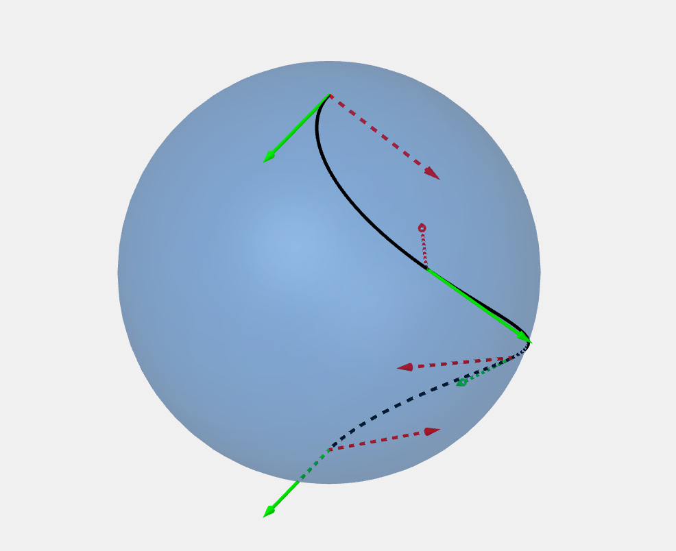
 Non geodesicGeodesic